Statistical inference –
the basics
The basic
logic of orthodox statistical inference is as follows: you try to determine the
probability that the structure of your data can be explained by a null model;
if this seems improbable, you infer that something more interesting is going
on. We will return in the last session to a discussion of whether this is
really the best approach, and what alternatives there are.
A simple
example:
At a reception in the Informatics forum you notice that of
the first 10 people to take wine, 8 choose the red. Is this evidence of a
significant preference for red wine in the Informatics population?
Rephrased: if there was no real preference (i.e. choice was random)
what is the probability of observing at least 8 out of 10 people choosing the
red?
Can describe this probability using the binomial
distribution:
for n
trials, each with probability p for
outcome X, the probability of getting k
occurrences of X =
![]()
In this case n=10, p=0.5 (if random) and k=8,9,10 (i.e. the chances for at least 8):

As probability > 0.05, more than 1 in 20, this is (by
convention) not considered significantly different from chance
To do this in R, you can use the distribution
function binom, where dbinom(x,n,p) gives the probability
density:
> dbinom(8,10,0.5)+dbinom(9,10,0.5)+dbinom(10,10,0.5)
Or use the binom.test()
function
> binom.test(2,10,p=0.5) #actually
the default is p=0.5 so you could just use binom.test(2,10)
But note
this gives different probability (often abbreviated as p-value, don’t confuse
with the parameter p=proportion), equal to twice the statistic we just
calculated. Why? Above, our null hypothesis was:
H0: there is no population preference
for red or white wine
and we
considered this against the alternative:
H1: there is a population preference
for red wine
This is
often called a 'one-tailed' hypothesis because it assumes the deviation from
chance could only be occurring in one direction. However, in advance of seeing
the data (and hence knowing that more people chose red) we might have no reason
to expect the deviation from the null hypothesis to be towards a preference for
red or white (we would have thought either preference to be equally noteworthy)
and our new alternative hypothesis would be:
H1: there is a population preference
for one colour of wine over the other.
Therefore a
more neutral test would ask ‘what is the probability of observing a split at
least as large as 8 out of 10 in favour of one or other colour of wine?’ This
means the cases we added up should also have included k=0,1,2; that is, the
cases where red wine was unpopular and the preference for white wine was at
least as strong as the preference we observed for red. By symmetry these are
equal to k=8,9,10, hence the correct test gives twice
the p-value. Try it out explicitly if you want to check. You can also
explicitly do a one-tailed binomial test;
> binom.test(8,10,0.5,"greater")
Note that a possible objection to this entire procedure is that
‘the first 10 people who took wine’ is not a random sample from the population
of Informatics – we can at best conclude something about the people who are
generally first in the queue for wine…
Exercise: if the proportion of
left-handed people in the population is 10%, and you observe in your group of
subjects who experience synaesthesia that 4 out of 10 are left-handed, should
you conclude left handedness is more common than usual in synaesthetes?
Note the
same method can be used on numerical data to do a sign test, a quick and simple test which makes minimal assumptions
about the population distribution (unlike some of the tests below). E.g.:
·
Twelve
(N = 12) rats are weighed before and after being subjected to a regimen of
forced exercise.
·
Each
weight change (g) is the weight after exercise minus the weight before:
1.7, 0.7, -0.4, -1.8, 0.2, 0.9, -1.2, -0.9, -1.8, -1.4, -1.8,
-2.0
> rats = c(1.7, 0.7, -0.4, -1.8,
0.2, 0.9, -1.2, -0.9, -1.8, -1.4, -1.8, -2.0)
Test whether
the proportion that has decreased weight is higher than expected by chance:
>
binom.test(sum(rats<0),length(rats))
But note
that this test has thrown away a lot of information in the data, i.e. the
actual size of the weight gains and losses, and as a consequence is less
powerful at detecting real differences. E.g. if the data looked like this:
1.7, 0.7,
-40.0, -18.8, 0.2, 0.9, -16.2, -10.9, -15.8, -19.4, -21.8, -25.0
You would
have the same conclusion from the sign test even though the data appears to
show much stronger evidence of significant weight loss. We will come back to
the issue of power later.
Frequency testing
Now, let's deal with the situation when we have categorical
data to analyse, in this simple example let's assume we collected information
about squirrels in the UK and in Poland.
Our raw data is in http://homepages.inf.ed.ac.uk/bwebb/statistics/squirrels.csv. First, download it to your working
directory, then, let's load it into R and see the first few rows:
> membership_data=read.csv(file='squirrels.csv')
> attach(membership_data)
> head(membership_data)
Then we can count representatives of 4 combinations of
country x fur colour and present the counts in a contingency table:
> contingency=table(country,fur)
> contingency
We want to test whether red squirrels are underrepresented in
the UK compared to Poland, i.e. how likely are the frequencies in the
contingency table to be due to chance.
First solution (which is appropriate for 2x2 contingency
tables and relatively small samples) is to use the Fisher exact test.
This will calculate exact probability of these frequencies occurring given the marginals, i.e. total number of red squirrels in the
sample, total number of British squirrels in the sample and total number of
squirrels in the sample.
We can do it manually, by reading the value directly from the
hypergeometric distribution
>
phyper(contingency['UK','red'],sum(contingency[,'red']),sum(contingency[,'grey']),sum(contingency['UK',]))
[1] 0.1761937
Or we can use the built-in function fisher.test,
which takes the entire contingency table as an argument and does the same
calculation under the hood.
> fisher.test(contingency,
alternative='less')
Fisher's Exact Test for Count Data
data:
contingency
p-value = 0.1762
alternative hypothesis: true odds ratio is less than 1
95 percent confidence interval:
0.000000 1.522656
sample estimates:
odds ratio
0.4743571
The alternative is chi square test, which approximates
probability with chi square distribution and is a preferred method for bigger samples, and can be
used bigger contingency tables.
Chi square statistic is calculated from the equation
![]()
where O stands for observed value and E
stands for expected value in each cell (based on marginal counts) and we sum
over all cells.
Then,
for any value of chi square statistic corresponding probability
can be read from a curve for a given number of degrees of freedom. These curves represent 1 – F(x)
where F(x) is a cumulative chi square
distribution function.
We could derive the expected values, perform the summation
and use the test statistic value in a cumulative chi-square distribution
function. However, we can let R do the work:
> chisq.test(contingency)
Pearson's Chi-squared test with
Yates' continuity correction
data: contingency
X-squared = 0.8668, df = 1, p-value = 0.3518
Interestingly, on default, Yates' continuity correction is
applied, it means that each O-E difference in the test statistic summation is
decreased by 0.5, i.e. the formula becomes
![]()
Hence the test
statistic becomes smaller and the resulting p-value is higher than if we run
the test without the correction:
> chisq.test(contingency,
correct=FALSE)
Pearson's Chi-squared test
data: contingency
X-squared = 1.5198, df = 1, p-value = 0.2177
Parametric testing
Note that
the basic idea above was that we compared the data to an expected distribution,
such the binomial distribution with a parameter given by the expected
proportion (e.g. p=0.5 under equal chance assumption). The idea can obviously
be generalised.
A simple
example:
If the
height of men in Britain is normally distributed with mean μ=175cm and standard
deviation σ=8cm, is a height of 185cm unusual?
We could ask
what is the probability of someone randomly chosen from this population being
exactly 185cm tall, using the probability density dnorm(x,mean,s.d.) - recall we used ‘rnorm’
in the previous session to get a random variable from a normal distribution.
> dnorm(185,175,8)
But as
before, the question is really about the probability of someone being at least
185cm tall, or taller. So we want to know the probability of falling in the top
tail of the distribution, which we can calculate as 1 - the cumulative
probability of the distribution up to 185, using the function pnorm:
> 1- pnorm(185,175,8)
An
alternative way of considering a height of 185 compared to a mean of 175 is to
ask about the probability of deviating 10cm from the mean. This is the
two-tailed rather than one-tailed question, as discussed above. To answer it
you need to add in the other end of the distribution, i.e. for heights below
165:
> 1- pnorm(185,175,8)+pnorm(165,175,8)
(Or more
simply, due to symmetry of the normal distribution, just double your previous
p-value). More typically, we compare the value of some statistic to the
standardized normal distribution μ=1, σ=0, by first doing a
Z-transform on the value (expressing each score in terms of how much it
deviates from the mean, in multiples of sd.)
![]()
> z=(185-175)/8
And compare
it to the standardised normal distribution (the default for the norm
functions).
> 1-pnorm(z)
Above we
mentioned that by convention, something that has a probability <.05 is
considered significantly different from expectation. You should keep in mind
that this means (a rather unimpressive) 1 in 20 – e.g., for heights, you are
going to encounter plenty of men in the UK who are ‘significantly’ different
from average, but it is unlikely someone’s unusual height would lead you to
reject the assumption that they come from the UK. So when scientific reports say something is
significant, you should not be too convinced. We will come back to this point
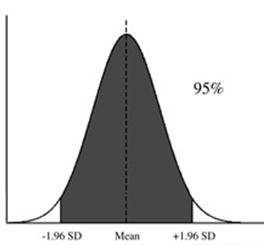
later. Meanwhile, it is handy to know that the z-value which cuts off 2.5% at
each end of the standardized normal distribution is +/-1.96. This is often
called the ‘critical value’ and can be obtained using:
>qnorm(.975) #
gives the 97.5 percentile for the normal distribution.
You can
check:
> pnorm(-1.96)+1-pnorm(1.96)
So in fact,
once you calculate a z-score, you can immediately see whether or not it falls
above or below the ‘critical value’
z=+/-1.96, and thus whether it is significant at p <.05. E.g. for the height
185, the z-score was 1.25, which is<1.96 so p>.05. We can also calculate
what deviation from average height would be considered ‘significant’, i.e. one
that is 1.96σ from the mean, or in this case 175+/-1.96*8, i.e. taller
than 190.6cm or shorter than 159.3cm. Another way to describe this is to say
that 95% of the UK male population have a height that falls in the range 159.3
to 190.6 cm.
Single sample tests
Let’s go
back to our previous simple example of data:
• Twelve (N = 12) rats are weighed
before and after being subjected to a regimen of forced exercise.
• Each weight change (g) is the weight
after exercise minus the weight before:
1.7, 0.7, -0.4, -1.8, 0.2, 0.9, -1.2,
-0.9, -1.8, -1.4, -1.8, -2.0
What we want
to do is use this sample to estimate the weight change that might be expected
in the population (an interesting question to also consider here is ‘what is
the population’? Strictly speaking we should only generalise to the rats from
which these were a random sample, e.g. the particular strain of rats in this
particular lab, but the motivation for the experiment is likely to be an
interest is generalising from rats to humans), and to say whether this is
significantly different from zero. A
possible estimate for the average weight change is the sample mean:
![]()
> mean(rats)
-0.65
(Though you
might want to check the distribution and decide if the mean is really
representative. For the moment we will proceed as if it is). We want to compare
the sample mean we have obtained to the expected distribution of sample means
under the null hypothesis that the population mean is zero. If we took repeated
independent random samples of size n from a population of mean μ and
standard deviation σ:
[1] The mean
of the population of sample means is equal to the mean of the parent population
from which the population samples were drawn.
[2] The
standard deviation of the population of sample means is equal to the standard
deviation of the parent population divided by the square root of the sample
size: σ/√n. This is sometimes called the standard error of the mean,
or s.e.
[3] The
distribution of sample means will increasingly approximate a normal distribution
as the sample size increases, whatever the underlying population distribution.
This is the Central Limit Theorem.
In this case
we have a (null) hypothesis for the population mean, i.e. μ =0, but we
don’t know σ. Let’s imagine for a moment that we do happen to have this,
say σ=0.8. Then for our sample size, n=12, the standard error of the mean
is 0.8/√12=0.23. We could then calculate the probability of the observed
mean just as we did above for heights. We are comparing the sample mean =-0.65
to a normal distribution (of sample means) with mean 0 and s.d.
= 0.23
> pnorm(-0.65,0,0.23)
Note again
this is one-tailed – it assumes we’re only interested in the probability of
values of the mean that are at least 0.65 below zero (weight decreases) but not
equally large values above zero (weight increases). We could double the value
to get the two-tailed result:
> 2*pnorm(-0.65,0,0.23)
This seems
pretty improbable, so we might want to ‘reject’ our null hypothesis, and
conclude our mean from the sample is a better estimate of the true value of the
population mean. In fact, we could put some probability bounds on this estimate
using the critical z-value 1.96 as before, by calculating that 95% of the
distribution of sample means will be within +/-1.96*s.e.
of the observed mean.

Thus in the
case of rat weights we have a lower and upper bound of the ‘likely’ value of
the mean:
> -0.65-1.96*0.23
> -0.65+1.96*0.23
This is
called the 95% confidence interval (C.I.). Strictly speaking it says that if we
kept taking samples of size n from the population with μ = -0.65,
σ=0.8, 95% of the means would fall between -1.1g and -0.19g. It is quite
useful as a summary statistic (which can be easily plotted on a graph) because
it essentially combines an indication of the size of the observed effect with a
significance test: if the value of our null hypothesis (here that μ=0) is
not contained within this interval then we know the observed mean is significantly
different from 0, p<0.05. By extrapolation we could calculate a 99% C.I., or any other
percentage we think appropriate, but as the percentage goes up (so our
‘confidence’ that we’ve bracketed the true mean increases) the interval will
get wider. Hopefully obvious is that the C.I. will get smaller as our sample
size n gets larger – the accuracy of our estimate will improve as we collect
more data.
The t-test
By now you
should be worried by the fact that we don’t actually know the population standard
deviation σ, we just used a number I made up. An obvious thing to do is
instead to estimate it from the sample standard deviation:
and divide
by √n to get the standard error of the mean:
> se.rats=sd(rats)/sqrt(length(rats))
We could now just plug that into our method
above to get a p-value and C.I. However, because we are using an estimate, we
need to make an adjustment, one that depends on the size of our sample: we
would expect the estimate to become closer and closer to the real population
standard deviation as we increase our sample size. Without going into detail,
instead of using a standard normal distribution Z, we use the T-distribution:
![]()
Where V is the chi-squared distribution with υ degrees of freedom (d.f.). The degrees of freedom is the sample size minus the number
of parameters estimated from the data, in this case having estimated the mean, d.f.=n-1.
The effect of this adjustment is to increase the size of the tails of the Z
distribution, gradually approaching the normal distribution as υ increases
(a general rule of thumb is that for d.f.>30
there is no practical difference in the resulting statistical calculations).
Using R, we
have the t() function
which works like the binom() and norm(), e.g. pt(x,df)
is the cumulative probability. However note that this is ‘standardised’ i.e. to
get the probability of a particular value we need to give it as input a
t-score:
![]()
And (unlike the Z distribution) it needs the d.f. parameter. In our example so
far, we want to find the t-value of the sample mean, compared to a mean of
zero, which is the sample mean divided by the standard error of the mean.
![]()
> t.rats
= mean(rats)/se.rats
> df =
length(rats)-1
> 2*pt(t.rats,df)
And in a similar way one can calculate a confidence interval,
using qt()
to obtain the critical value of the t distribution.
> qt(.975,11)
But to save time, you might guess that R already has a
function to do a t-test based directly on the data vector, which also produces
a 95% C.I.:
>t.test(rats) # you can specify a value other than zero for
the population mean to test against with t.test(x,mu=y)
As a matter of interest you might like to compare the p-value
result here to that we would estimate from the normal distribution (using pnorm), but now using the estimated s.d. from the sample
(=1.25) compared to the hypothetical s.d. of 0.8 that
we used above. The result should be an underestimate of the p-value obtained
from the t-test.
Alternatives to the t-test
Above, we used the Central Limit Theorem to justify the
assumption that our sample mean comes from a normal distribution (or adjusted
t-distribution). But the CLT holds in the limit; if we have a small sample, we
can’t make this assumption. However, the distribution of sample means from a
normally distributed population will always be normal; in this case we are
safe. Hence, it is often stated that we
can only apply a t-test if our data comes from a normal distribution. This
is probably better stated as:
If the data do not appear normally distributed (see
last session) and the sample size is small, results from a t-test may be
misleading, and an alternative ‘non-parametric’ test should be considered.
On the other hand, for a small sample, it may be hard to
judge whether the distribution is normal. For rat weights in particular, we
might argue that each measured weight difference is already the sum of a wide
number of biochemical random factors, and hence we have a prior expectation
(via the CLT) that they should be normally distributed.
We’ve already looked at one non-parametric test above, the sign test, which compared the values in
our rat data to 0 by simply counting how many data points fell each side of
zero.
A second alternative that uses a bit more information from
the data is the Wilcoxon test. The
basic idea (common to many non-parametric tests) is to
use the ranks of the data rather than the numerical values themselves. As a
consequence it is also appropriate to use this test when the data themselves
are, in fact, ranks, e.g. as may typically result from survey data. The
procedure is actually simple enough to do by hand, see e.g. here: but can also be done in R:
> wilcox.test(rats,mu=0)
However note this test
still assumes the data is symmetric (around the median) so may not be suitable
for certain kinds of departure from a normal distribution.
A third alternative is to use bootstrapping. The simple idea here is that our best estimate of
the population distribution is that it is the same as the sample distribution.
So we use that sample data to generate a distribution of sample means, by
taking repeated samples with replacement from our original data and calculating
the mean.
> boot.rat =numeric(1000)
> for (i
in 1:1000) boot.rat[i] =
mean(sample(rats,replace=T))
> hist(boot.rat) # have a look at this distribution
> sd(boot.rat) # compare this to the standard error of the mean calculated above
We can then
calculate a 95% confidence interval directly from this distribution, from the
.025 and .975 percentiles
> boot.rat=sort(boot.rat)
> boot.rat[c(25,975)]
Note that we
also have an estimate of the mean:
> boot.rat[500]
And that the
bootstrapped C.I. is potentially assymmetric around
the mean, unlike the standard forms of C.I. calculated above.
Tests with two samples
A common
experimental design will have a dependent variable, or response, measured under
two (or more) conditions, for example, with one group getting treatment and the
other acting as a control. So we are interested in whether there is a
significant difference between the response of the
groups.
Crucially
there can be two different experimental designs with two groups: paired and
unpaired. E.g. paired design occurs when the same participant is tested under
both conditions (sometimes called ‘repeated measures’); but it includes any
design where there is a logical matching between each score in one group with a
corresponding score in the other group. Unpaired designs are sometimes called
independent designs.
The easy way
to avoid the mistake of analysing a paired design as an unpaired design, or
vice versa, is to realise that the two samples of a paired design can be made
into one sample by taking the difference of each pair, and then testing if the
mean difference is equal to zero (using the single sample methods discussed
above). The only reason not to do this would be if your data values are not
interval data, e.g. represent ranks, in which case taking differences is
misleading – then you should do a non-parametric test anyway (e.g. Wilcox.test() with the flag paired=T).
Variance of 2 samples
For an
unpaired, or independent design, most statistical tests to compare the 2 means
assume equal variance within each sample. We can test this assumption by
comparing the ratio of the variances to the F distribution, which is defined as
the ratio of two independent Chi-square distributions divided by their degrees
of freedom. The Chi-square
with k d.f. is the
distribution of the sum of squares of k independent random normally distributed
variables. N.B. the F-ratio will become key when we
get to ANOVA tests.
Fisher’s F Test
·
Divide
the larger variance by the smaller one - variance ratio
·
Determine
the degrees of freedom, which will be [(n1-1),(n2-1)] where n1 and n2 are the
sample sizes for the samples with larger and smaller variances, respectively
·
Find
p-value for F statistic using pf() function
e.g.
> f.test.data =read.table("garden.txt",header=T) ##
find f.test.data
> attach(f.test.data) ## attach f.test.data
> names(f.test.data) ## list the names of
f.test.data
[1] "gardenB"
"gardenC"
> var(gardenB) ##
Compute variance for gardenB
[1] 1.333333
> var(gardenC)
## Compute variance for garden C
[1] 14.22222
Variance gardenC is much bigger than var gardenB,
so:
> F.ratio=var(gardenC)/var(gardenB)
> F.ratio
[1] 10.66667
1 or 2-tailed? 2 in this
case – no expectation as to which would have higher variance
> 2*(1-pf(F.ratio,length(gardenC)-1,length(gardenA)-1))
[1] 0.001624199
This is a
small probability, so the hypothesis that the variances are equal is rejected.
There’s a quicker version:
> var.test(gardenB,gardenC)
T-test
The test statistic is the number of standard errors by which
the 2 sample means are separated:
For
independent variables, variance of the difference of means is sum of separate
variances. Not true if variables are correlated (e.g. unlikely to be true in
paired design, hence mistakenly analysing a paired design this way will
overestimate the s.e., and
underestimate t).
Carrying out the t-test
We’ll use
the garden data in this example – however note (relative to last week’s
discussion) this means that we are assuming the ten measurements for each
garden are independent (e.g. they were not taken on the same days). We are
interested in whether the ozone levels differ between garden A and garden B.
1. Set out hypotheses
H0: There is no difference
between the two means
H1: There is a significant
difference between the 2 means
2.
Decide whether one or two-tailed, decide significance value, and
establish degrees of freedom in each sample; use these to find a critical value
for t
e.g.
2-tailed test; p=.05; for garden
data, d.f.
in each = n-1=9, total df = 18
> qt(.975, 18)
[1] 2.100922
So in this
case the test statistic (t) must
exceed 2.1 in order to reject H0 – that the 2 means are not
significantly different at the .05 level of significance.
3. Attach data frame (if you haven’t
already)
> t.test.data=read.table("gardens.txt",header=T)
> attach(t.test.data)
> names(t.test.data)
[1] "gardenA"
"gardenB"
4. Visualise the data
> ozone=c(gardenA,gardenB)
> label=factor(c(rep("A",10),rep("B",10)))
> boxplot(ozone~label,notch=T,xlab="Garden",ylab="Ozone")
Variability appears similar in both samples – range (whiskers), inter-quartile range (IQR, size of boxes) are
fairly similar. The notches show +/-1.58*IQR/sqrt(n) which is an approximate 95% confidence
interval for the median. If the notches don’t overlap, the medians are probably
significantly different.
5. Long-hand t-test
a. Calculate variability for each sample
(if they look very different, should check equality with F test, as above, and
should not proceed if this is significant)
> varA=var(gardenA)
> varB=var(gardenB)
6. Calculate the value of t:
Student’s t is difference between 2
means divided by the square root of the sum of (the variance of each sample
divided by its sample size)
> (mean(gardenA)-mean(gardenB))/sqrt(varA/10+varB/10)
[1] -3.872983
7. Interpret the value of t.
a. Ignore the minus sign – look at the
absolute value of the test statistic
- A value of 3.87 exceeds the critical value of
2.10(above)
- Therefore we can reject the null hypothesis in
favour of the alternative hypothesis: there is a significant difference between
the 2 means
8. Calculate an exact p-value – the probability that this, or
more extreme, data / differences would be observed under the null hypothesis
> 2*pt(-3.872983,18)
[1] 0.00111454
P < .001; it is highly unlikely these
differences occurred by chance
Or – use the built-in t-test function:
> t.test(gardenA,gardenB)
Welch Two Sample t-test
data: gardenA and gardenB
t = -3.873, df = 18, p-value = 0.001115
alternative
hypothesis: true difference in means is not equal to 0
95 percent confidence interval:
-3.0849115 -0.9150885
sample estimates:
mean of x mean
of y
3
5
Garden B was found to have a significantly higher mean ozone
concentration than garden A (means: 5.0, 3.0 p.p.h.m,
respectively). t(18)=-3.873; p<.001
Note that
the “Welch” test applies a correction for potentially unequal variance.
Power, effect size and
sample size
So far we’ve
mentioned several times that by convention, a probability <.05 for observing
data under the null hypothesis is taken as significant evidence against the
null hypothesis. More formally this is called the ‘Type I error rate’ or
‘α’ level, where a ‘Type I’ error would be to reject the null hypothesis
when it is, in fact, true. ‘Type 2’ error would be to fail to reject the null
hypothesis when it is, in fact, false. This is called the ‘β’ level, and
often discussed as power=1-β. I.e. the power of a statistical test is its
ability to correctly detect a false null hypothesis. In general there will be a
trade-off between α and β, which depends on the size of the sample,
the size of the effect (known as δ), and the variance in the data.
What this
means is that if you know 4 of these 5 variables, you can determine the 5th.
E.g. after doing a test, you can calculate what its power was (see
here for a discussion of how (and how not) to interpret this). If you have failed to reject the
null hypothesis, a low power might suggest that you simple failed to detect a
difference that does, in fact, exist – because the effect is small, or the
variance is large, or you did not collect enough data, or all of these. Perhaps
more usefully, before doing an experiment, you
can estimate the sample size required to observe, at a given α and
β level, an effect of a certain size, given an estimate of the likely
variance. For example, if you expect the difference between the means to be at
least 2, and the variance around 10, and want to ensure you have power=0.8
(again this is the conventional figure) using a conventional α=0.05, then
you can use:
> power.t.test(type="two.sample",delta=2,sd=sqrt(10),power=0.8,
sig.level=0.05)
-to find out
that you need n=40. Note it is much better to do this before running your experiment: to make sure you collect enough
data to see the effect if it exists; to not waste time collecting a lot more
data than necessary to see the effect exists; or to redesign your experiment
(to reduce variance or increase effect size) so that you don’t have to collect
so much data. However it does require an estimate of the effect size and
variance, before you run the experiment. Sometimes you may be able to estimate
these from previous experiments in the literature. Sometimes a pilot experiment
may help (using bootstrapping on pilot data to estimate the variance is a
useful technique). What is really not
a good idea is to start an experiment not knowing how much data you should
collect, running statistical tests as the data comes in, and then stopping when
the result is significant: see here for a quick demonstration and
discussion of the misleading results this can produce.
Note also
that there may be good reason for varying from the conventions for α and
β, depending on the potential consequences of making a Type I or Type II
mistake.
Effect size is a measure of the strength of the
difference expected, or retrospectively, observed. An absolute effect size
(e.g. difference between the means) might sometimes determine the practical
(rather than statistical) significance of your result. E.g. if you were looking
at the effects of various diets, and found one diet with radically reduced
calories produced a 10 gram weight loss over a year compared to a control diet,
that might be robustly statistically significant, but not actually of much
practical or scientific significance. A standardised effect size measure, such
as Cohen’s d, compares the difference in the means to the variance in the data,
and is sometimes used to loosely classify an observed effect as ‘small’,
‘medium’ or ‘large’.
![]()
Where s is
the pooled standard deviation of the samples (or if we have assumed these are
equal, the s.d. for either). So for example in our
garden data above, the effect size is
> d = (mean(gardenA)-mean(gardenB))/sqrt(varA)
which comes
out as -1.7, meaning the means differ by 1.7 standard deviations. Cohen
suggests that d=0.2 be considered a 'small' effect
size (an effect that probably means something is really happening in the world
but it takes careful study to see it), 0.5 represents a 'medium' effect size
and 0.8 a 'large' effect size (an effect big or consistent enough that you
could probably see it without statistics).
Although
this is still somewhat arbitrary, note that this approach is better justified
than trying to conclude you have a ‘strong’ effect from the size of the p-value
– the logic of the orthodox statistical test implies that however small the
difference between the means, a large enough sample size will result in
rejecting the null hypothesis for any level of α you choose. We will come
back to this point in session 5.
To get a
better feel for the trade-off between power, sample size and effect size try
this demonstration:
First we'll set up vectors with a range of
effect sizes (the difference between the means relative to the variance in the
data) and power values
> d
= seq(0.25,1.5,.05)
>
nr = length(d)
>
p = seq(.4,.9,.1)
>
np = length(p)
Now we can compute required sample size for
all values of d and power
> samsize = array(numeric(nr*np), dim=c(nr,np))
>
for (i in 1:np){
for (j in 1:nr){
result = power.t.test(type="two.sample",delta=d[j],
sd=1,power=p[i], sig.level=0.05)
samsize[j,i] = ceiling(result$n)
}
}
Finally, we set up a graph to visualise the
results
> xrange = range(d)
> yrange = round(range(samplesize))
> colors = rainbow(length(p))
> plot(xrange, yrange,
type="n", xlab="Difference between
means delta", ylab="Sample Size n" )
For each value of power we add a curve in a
different colour
>
for (i in 1:np){
lines(d, samplesize[,i], type="l", lwd=2,
col=colors[i])
}
Also, we can add a legend
>
legend("topright", title="Power",
as.character(p), fill=colors)
Now you can see how required sample size depends
on the difference between means which we expect and the power value which we're
aiming to achieve.
NOTE
ABOUT INSTALLING PACKAGES
There is a
package which extends power analysis to many other statistical tests, however,
it is not supplied in the base installation of R. (This is a common situation
with R)
There is a central repository of R packages
(CRAN) which allows us to install and load packages in a standardised way.
Basic
command for that is install.packages('package_name')
to install it, and library(package_name) to load it, dependencies are resolved automatically.
However, if
you're working on a machine where you don't have admin rights (e.g. DICE), you will need to install packages to a local folder, in
order to set it up type:
> system('mkdir ${HOME}/localRlibraries')
> system('export R_LIBS=${HOME}/localRlibraries')
These two
UNIX commands executed through R will create a folder for local R libraries and
then point an environmental variable to this folder.
Then we can
install a package and specify the repository to use (this only needs to be done
once, subsequently you can omit repos argument)
> install.packages('pwr', repos='http://star-www.st-andrews.ac.uk/cran/')
Finally, we load packages with library
command
> library(pwr)
You can explore contents of this
package if you have time.