Introduction

ML stands for “MetaLanguage”. Robin Milner had the idea of creating a programming language particularly adapted for writing applications that would process logical formulae and proofs. This language would be a meta-language for manipulating objects representing formulae of the logical object language.

The first ML was the meta-language of the Edinburgh LCF proof assistant. It turned out that Milner’s meta-language became, with later additions and refinements, a versatile and innovative general-purpose programming language. Today there are many languages that adopt many or all of Milner’s innovations. Standard ML (SML) is the most direct descendant of the original, CAML is another, Haskell is a more-distant relative. In this note, we introduce the SML language, and see how it can be used to compute some interesting results with very little programming effort.

In the beginning, you were told that a program is a sequence of instructions to be executed by a computer. This is not true! Giving a sequence of instructions is just one way of programming a computer. A program is a text specifying a computation. The degree to which this text can be viewed as a sequence of instructions varies from programming language to programming language. In these notes we will write programs in the language ML, which is not quite so explicit as languages such as C and Pascal about the steps needed to perform a desired computation. In many ways, ML is simpler than Pascal and C. However, you may take some time to appreciate this.

ML is primarily a functional language: most ML programs are best viewed as specifying the values we want to compute, without explicitly describing the primitive steps used to achieve this. In particular, we will not generally describe (or be concerned with) the way values stored in particular memory locations change as the program executes. This will allow us to concentrate on the organisation of data and computation, without becoming mired in detailed housekeeping.

ML programs are fundamentally different from those you have become accustomed to write in a traditional imperative language. It will not be fruitful to begin by trying to translate between ML and the more-familiar paradigm — resist this temptation!

We begin this chapter with a quick introduction to a small fragment of ML. We then use this to investigate some functions that will be useful later on. Finally, we give an overview of some important aspects of ML.

It is strongly recommended that you try some examples on the computer as you read this text.¹

An ML session

We introduce ML by commenting on a short interactive session. In the text, human-computer interactions are set in typewriter font. Lines beginning with a prompt character — > or # — are completed by the human; other lines are the ML system’s responses.

Evaluating expressions If the user types an expression, the ML system responds with its value — this makes your workstation into an (expensive) calculator.

> 4.0 * arctan(1.0);   val it = 3.141592654 : real

In this example, an expression is evaluated to compute the real number, π.

Naming values A value declaration, introduced with the keyword val, allows us to give a name of our choice to the value of an expression. The value declaration:

> val pi = 4.0 * arctan 1.0;   val pi = 3.141592654 : real

gives the name, pi, to the value, π, for use later in our ML session.

Declaring functions ML provides a number of built-in functions, such as arctan; an ML program extends this repertoire by declaring new functions. To declare a function, toDegrees, that converts an angle in radians to degrees, we use the keyword fun, followed by the mathematical definition of the function:

> fun toDegrees(r) = 180.0 * r / pi ;   val toDegrees = fn : real -> real

We can use this just like any built-in function:

> toDegrees(1.0);   val it = 57.29577951 : real

—one radian is approximately 57.3 degrees.

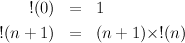
Recursion A function defined using fun may be recursive. Here we declare the factorial function:

>  fun fact(0) = 1   #  |   fact(n) = n * fact(n-1);   val fact = fn : int -> int

In this example, the declaration consists of two clauses. The first clause applies when the argument is zero, the second in every other case; so and so on. The factorial of 40 is a large number:

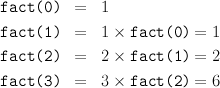
> fact 40;   val it = 815915283247897734345611269596115894272000000000 : int

Summary This example session demonstrates several key ideas:

• We evaluate expressions to find their values.
• Values may be named so they can be re-used without recomputation.
• To extend the range of expressions we can evaluate, we declare functions.
• Recursion allows us to perform repetetive computations.

Basic ML

A program consists of a sequence of declarations:

value declarations

of the form val 〈 name〉 = 〈 expression〉, and

function declarations

of the form fun 〈 name〉 〈 pattern〉 = 〈 expression〉.

in addition, a function declaration may have several clauses, separated by | . Identifiers, such as arctan, x, pi, +, and *, are used as names; fun, val, =, |, and ; are keywords — they have special meanings in ML.

We will introduce other ML constructs in due course, but first we use this fragment to investigate the relationship between the size and height for various shapes of tree.

Trees and counting

Trees will figure largely in these notes. Here we use recursive functions to compute various “vital statistics” of a tree. These will be useful to us in due course. Later, we will represent trees themselves as data values, and write functions that build and transform trees; we will study tree-based algorithms in some detail. For now, we use trees to provide some interesting counting problems, and restrict ourselves to numeric calculations in our simple fragment of ML. We will write ML functions to count the numbers of leaves and nodes in trees of various shapes.

Binary Trees

A binary tree is one in which each internal node has exactly two children (we call them left and right, for convenience).

Full Trees A binary tree is full if, at each internal node, the left and right subtrees grow equally; in particular, they are both full and have the same height. We start by counting the leaves of a full binary tree. We introduce a notation b(n), say, for the number of leaves in a full binary tree of height n, and write down a couple of obvious equations:

A tree of height zero is just a single leaf; the number of leaves in a tree of height n + 1 is the sum of the numbers of leaves in its two subtrees (both of height n). Here is an ML function to compute b(n)

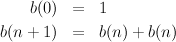
fun B(0) = 1  
  | B(n) = B(n-1) + B(n-1);

The relation to the mathematical equations is just like that for the factorial function. This is an obviously correct way to compute b(n), but it is particularly inefficient. We’ll return to the issue of efficiency later.

Balanced Trees

A tree is unbalanced if it grows unequally. In the most unbalanced binary tree, one child of each internal node has zero height. We call such a tree a spine. The number S(n) of leaves in a spine of height n is given by the following equations:

The corresponding ML function definition is

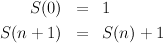
fun S(0) = 1  
  | S(n) = S(n-1) + 1;

Again, efficiency will come later; this is not the most effective way to compute S(n)!

We say a tree is balanced if, at any node, the heights of the two subtrees differ by at most 1.

Now consider a balanced tree, where the height of each right subtree is, if possible, exactly one less than the height of its sibling, left, subtree. Let F(n) be the number of leaves in a slightly unbalanced tree of height n.

This function should be vaguely familiar; here is the corresponding ML declaration:

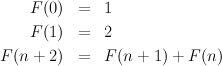
fun F(0) = 1  
  | F(1) = 2  
  | F(n) = F(n-1) + F(n-2);

Bushy Trees

In an n-ary tree, each internal node has n children. A full n-ary tree of height h has T_n(h) = n^h leaves.

fun T(n,0) = 1  
  | T(n,h) = n * T(n, h-1);

Binomial Trees

Now we consider a more complex, and more interesting, example. A binomial tree, B_n, of height n has a root node with n children; these children are the roots of the n binomial trees B_n-1…B₀. Notice that, by this definition, B₀ is just a leaf.

Now let us write B(n) for the number of nodes in the binomial tree B_n

Here we add one (for the root node) to the sum representing the nodes of the n children. Following the model of the function given earlier for summing squares, we can compute B(n) as follows

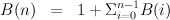
fun B(n)  = 1 + SB(n)  
 
and SB(0) = 0  
  | SB(n) = B(n-1) + SB(n-1);

Here we declare two mutually recursive functions; the declarations of B and SB depend on each other. Mutually recursive declarations in ML are conjoined using the keyword and.

Exercises

Expressions

In a functional programming language, values are computed by evaluating expressions.

Functions and application Most expressions are formed by applying functions (such as arctan and *) to arguments. Function application is normally indicated by prefix juxtaposition, i.e. we may type sqrt 2.1 to apply the square root function to the argument 2.1. Parentheses are not needed. However, parentheses may be placed around any expression, so we could also type sqrt(2.1), or (sqrt 1.0) —or even sqrt(((2.1))), or (sqrt) 1.0. These are all equivalent: evaluating any one of these expressions provokes the response

val it = 1.449137675 : real

Infix functions For some functions, infix notation is used; for example, to add 1 and 3, we evaluate the expression 1 + 3 . Many binary operations are provided as infix functions. Different infix functions may have different precedences; for example, multiplication has a higher precedence than addition. ML expressions are just like algebraic expressions. As in algebra, parentheses may be used to bracket sub-expressions:

> (3 * 4) + 2 ;   val it = 14 : int   > 3 * (4 + 2) ;   val it = 18 : int   > 3 * 4 + 2 ;   val it = 14 : int

Prefix function application takes precedence over infix function application.

> arctan 1.0 * 4.0;   val it = 3.141592654 : real   > cos(it/3.0);   val it = 0.5 : real

We normally omit parentheses unless they clarify, or are needed to determine, the intended order of evaluation in a complex expression.

Conditional expression A conditional expression chooses between two values on the basis of a Boolean condition:

fun maximum (x,y)= if x >= y then x else y

The conditional expression has the form if 〈 condition〉 then 〈expression₁〉 else 〈expression₂〉. The condition should be an expression of type bool. One or other of the expressions, expression₁ and expression₂, is evaluated, depending on the value of the condition. These two expressions must both have the same type, so that the type of the conditional expression is well-defined.

Types

ML is a strongly-typed language: each function expects an argument of a particular type, and returns a particular type of result. When we evaluate an expression, the system responds with its value and its type. If we supply the wrong type of argument to a function, the system complains:

> size 1 ;   Error- Can’t unify string with int  Found near size(1)   Exception static_errors raised

The function, size, expects a string as argument; it doesn’t make sense to apply it to an integer. To the novice, ML may appear overly particular about types; however, it is instructive to notice that, once you have constructed a well-typed program, ML programs are often ‘right first time’.

Basic Types There are four basic types in ML:

int

— a type representing integer values. The usual arithmetic operations — +, -, *, div and mod, equality and ordering relations — =, <=, >=, <>, are defined on the integers. Because operations in ML are typed, we distinguish unary minus, ~ : int -> int, from binary subtraction, - : int * int -> int. We also use ~ for negative integer constants.

real

— a type representing real values. These are different from the integers. There are no implicit coercions between the two; use the functions real and floor to convert between them. However, many arithmetic and ordering operations are overloaded: an instance of these operations may apply either to reals or to integers. Real division, /, is distinguished from integer division (div); a real constant is distinguished from an integer by a decimal point, an exponent, or both. ML also provides a basic set of analytic and trigonometric functions on reals.

string

— a type of (8-bit-)character strings. Strings constants are delimited by double quotes ("...."); various escape sequences are defined to allow you to include control characters in the string ??. Operations on strings include size, concatenation, ?, equality, =, and the overloaded ordering operations, as for reals and integers.

bool

— a type of Boolean truth values, consisting of the constants true and false. This type is used in the conditional expression that will be introduced in the next section.

Function types In ML, functions are values, so we can use the system to find the type of a function.

> size ;   val it = fn : string -> int

The expression size has a value that has no useful printed representation (fn merely signifies that it is a function). However, it is very useful to know its type; string -> int is a function type: the type of functions that, like size, take an argument of type string and return a result of type int. We will often draw diagrams showing functions as arrows going from one type (the argument type) to another (the result type): for example,

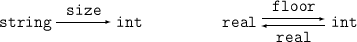
The symbol -> in the notation for a function type is derived from the arrows in these diagrams.

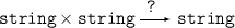
We can also find the type of an infix function²:

> ˆ ;   Warning- (ˆ) has infix status but was not preceded by op.   val it = fn : string * string -> string

The type of the operation tells us that it takes a pair of strings as argument, and returns a string as result. In a diagram, we write the argument type as a product

Declarations

ML provides a number of built-in functions, and constants for the basic types. An ML program is a sequence of declarations that extends this repertoire. Declarations give names to new values and functions.

Identifiers and binding

Identifiers in ML are names that stand for values. Evaluating an expression binds the identifier, it, to the result of the evaluation. We can then use “it” as a name, to refer to the value in another expression.

> 2;   val it = 2 : int   > it + it;   val it = 4 : int   >  it + it;   val it = 8 : int   >  it + it;   val it = 16 : int

Value declarations A value declaration, introduced with the keyword val, allows us to give a name of our choice to the value of an expression.

> val pi = 4.0 * arctan 1.0;

The general form of a value declaration is

Keywords cannot be used as names; for a list of keywords, and for the rules for generating identifiers, see ?? and ??.

Function declarations Function declarations are introduced with the keyword fun. The syntax is similar to that for value declarations, except that you have to specify pattern for the formal parameters:

The expression on the right-hand side can then refer to the parameters. We can use a single variable as a pattern:

fun twice(x) = 2 * x;

A pattern may also introduce a number of formal parameters:

fun modulus(x,y) = sqrt(x*x + y*y);

When the pattern is a single variable, the parentheses may be omitted.

> fun toDegrees r = 180.0 * r / pi ;   val toDegrees = fn : real -> real

This declaration binds the identifier, toDegrees, to a function that converts an angle in radians to degrees.

We will see more sophisticated examples of patterns shortly.

Declaring infix functions To declare an infix function, we first declare an identifier to be infix, and then use infix notation in the function declaration. Here is an example, we introduce an identifier ||:

infix ||;     fun x || y = sqrt(x*x + y*y);

Type constraints The system tries to work out the types of all expressions. For example, in sqrt(x*x + y*y), because sqrt is defined on reals, the system can infer that + and * refer to real addition and multiplication; in 2 * x, the integer constant 2 shows that integer multiplication is intended. Because some operations are overloaded, type inference is not always possible .Consider the definition “fun double(x) = x + x;” The fact that + is applied to x constrains x to be either an int or a real; but the compiler needs more information, to decide which kind of addition to perform. A type constraint can be used to provide the required information. Given an expression exp, and a type typ (e.g. int) then exp:typ is also an expression. Thus, we can type

fun double(x) = (x + x) : int;

to resolve the uncertainty by constraining the result type. Patterns may also be constrained in a similar way: we can type

fun double(x) : int = x + x;

to constrain the result type; and

fun double(x:int) = x + x;

to constrain the argument type.

In any case, when using ML you will find that the context normally provides all of the type information needed by the system. Type constraints are rarely necessary; however, they often make code easier to read. Redundant type constraints can provide useful documentation. Since compilation will fail if a type constraint is incompatible with the inferred type, this form of documentation will always match the actual code.

Polymorphism Consider the declarations:

fun I x        = x   fun swap(x, y) = (y, x)

Surprisingly, types for these operations can be inferred by the ML compiler:

val I = fn : ’a -> ’a   val swap = fn : ’a * ’b -> ’b * ’a

The primes, “’”, indicate type variables. The identity function, I, can be applied to an argument of any type, A, and will return a result of the same type; swap can be applied to a pair of type A×B, and will return a result of type B ×A. We say these functions are polymorphic (from the Greek) because they can take many forms: for example, I can be used as a function of type int -> int or as a function of type real -> real.

Recursion

A function defined using fun may be recursive, as in

fun fact 0 = 1  
  | fact n = n * fact (n - 1);

This definition uses two clauses separated by | (which is a keyword, read or). The first clause uses a constant, 0, as a pattern; this pattern is only matched when the argument is zero. When evaluating a function call, the first clause that matches is used, so the second clause will be applied for all non-zero arguments. The ML definition of factorial corresponds closely to the mathematical definition:

However, you should notice the following difference: in mathematical notation we use n + 1 as a pattern signifying that this case applies to natural numbers greater than zero; in ML there is no such pattern — we rely on the order of the patterns to get the same effect. The second clause of the ML function definition is only applied when the pattern of the first clause, in this case the constant 0, has failed to match the argument.

Recursion is used extensively in functional programs, taking the place of constructs such as while and for loops in an imperative language. For example, to compute the sum of the squares of the first n natural numbers

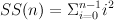
we write the following ML functions

fun square n : int = n * n;  
 
fun SS(0) = 0  
  | SS(n) = square(n-1) + SS(n-1);

The keyword and may be used to combine function declarations, allowing them to be mutually recursive:

fun even 0 = true  
  | even n = odd (n-1)  
and odd  0 = false  
  | odd  n = even(n-1);

Of course this isn’t a particularly sensible way of defining even and odd!

Equational reasoning

Functional, or applicative, programming is a programming style based on defining and applying functions. One advantage of functional programming is that functions may be viewed as mathematical objects, about which we can reason equationally. In other words, we can use algebraic manipulations to reason about our programs.

Infix notation can often make algebraic laws much easier to see. For example, the operation || introduced earlier is both associative,

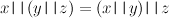
and commutative,

Sometimes diagrams can give a vivid picture of an equation relating two ways of computing the same value. We give a simple example, to introduce the idea of a commuting diagram. If we make the declarations

fun stutter s = s ˆ s   fun twice   x = 2 * x

then, for any string, s,

We can express this equation using a diagram

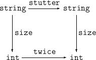
Following the arrows around the square in either direction gives the same result; we say the diagram commutes.

Scope

In ML, variables are statically scoped, just as in C and Pascal. So far, we have seen two ways to introduce variables: at the top level, or as arguments to functions. A top-level variable is in scope until the end of the program, although a hole may be introduced in the scope by the subsequent declaration of a variable with the same name. The scope of a variable introduced as a formal parameter, by a pattern in a function declaration, is confined to the body of the function, just as you would expect. To reinforce these points, consider the following example

val a = 1;  
 
val b = 2;  
 
fun f a = a + b;  
 
val b = 3;  
 
f b;

In the body of the function f the variable a refers to the formal parameter, and b has the value 2. The declaration following this introduces a new variable that just happens to have the same name as an existing one. It doesn’t alter the behaviour of f, i.e. it shouldn’t be read as an assignment to b. The result of the application should be 5 — is this what you expected?

Declarations introduced using val and fun are processed sequentially. The and keyword may be used to process declarations “simultaneously”. For example, if x is currently bound to 1 and y to true, then the declaration

val x = y and y = x;

would result in x being bound to true and y to 1, whereas

val x = y val y = x;

would leave both x and y bound to true. Note that, as in the earlier examples, you should view these definitions as introducing new variables, albeit with the same names as some existing variables, rather than as a sequence of assignments.

To allow the declaration of recursive functions, there is a subtle, but crucial, difference between the scopes of identifiers introduced by val and fun declarations. When we bind an identifier, val-id, using a val declaration, any occurrence of val-id in the body of the declaration refers to the previous binding of val-id: the scope of the new binding of val-id starts after the declaration. However, when we bind an identifier, fun-id, using a fun declaration, occurrences of fun-id in the body are treated recursively: the scope of the new binding of fun-id includes the body of the declaration.

Combining declarations

So far we have introduced SML programs consisting of a sequence of “top-level” declarations. We now look at more interesting ways of combining declarations. To make the scope of a declaration local to an expression, or to another declaration we can use

let 〈declaration₁〉 in 〈expression₂〉 end

and

local 〈declaration〉 in 〈declaration〉 end

Note the difference between let and local — and the terminating end required by each construct, which is easy to forget. We give examples using these constructs. The mathematical definition of the factorial function applies to natural numbers; if we allow our straightforward transliteration to be called with a negative argument, it loops forever. We could make a test at every recursive call,

fun fact 0 = 1  
  | fact n =  
    if n < 0 then error "negative n"  
             else n * fact (n-1);  

but this is not necessary

local  
    fun ffact 0 = 1  
      | ffact n = n * ffact (n-1)  
 in  
    fun fact n =  
        if n < 0 then error "negative n"  
                 else ffact(n)  
end;  

In ML each variable must be declared before it is used. The same rule is enforced in Pascal and C — but a number of other functional languages (in particular, some dialects of lisp) have a different rule. The ML rule allows programs to be constructed bottom-up, but sometimes makes it trickier to develop them top-down, or at least to present the top-down design steps explicitly. The modules facility, covered later in the course, is designed to support top-down development.

A Computational Model

ML uses “call-by-value” evaluation order. The general form of an application is exp₁ exp₂. To evaluate such an expression the system performs the following steps:

1. exp₁ is evaluated to produce a function. exp₁ is often a variable, such as fact, and so this part is usually simple.
2. exp₂ is then evaluated to produce a value.
3. The function body is then evaluated after performing pattern matching on the argument value.

The important thing to note is that the argument is always evaluated before the function body. This is sometimes inefficient, as in

fun silly x = 0;  
 
silly(3+2);

Here the evaluation of 3 + 2 is redundant. However, such cases are rare. Evaluating the body before the argument has been simplified carries its own performance penalties. We shall see how to simulate such a “lazy” evaluation strategy later in the course.

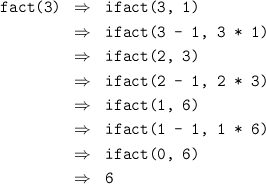
Using call-by-value, it is easy, if tedious, to expand out the application of a function to investigate the run-time behaviour. For example, given the definition of fact from Practical 1, we can simulate the execution of fact 3 as follows:

Note how the multiplications get delayed until the recursion “bottoms out”. We need to store these pending calculations somewhere (e.g. on the stack) and so the amount of storage required to evaluate fact n will be proportional to n. We can make the function more efficient (but more obscure) by exploiting the associativity of *. For example, we know that

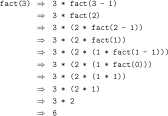
If we perform this rearrangement at each step then we won’t need to use the stack to save the pending multiplications. The following version of the factorial function performs this optimisation:

local fun ifact(0, p) = p  
        | ifact(n, p) = ifact(n-1, n*p)  
   in  
      fun fact n = ifact(n, 1)  
  end;

Here, ifact(n,x) = n! × x. The evaluation of this version of fact uses constant space:

This recursion has a special form: when a recursive call of the function is made, the caller returns the result of the recursive call directly, without further comupation; we say the call is tail-recursive, or iterative. In the original version of factorial the caller had to perform a multiplication using the result of the recursive call. Tail-recursive function calls can be implemented very efficiently. For example, a function tail-recursively calling itself can be compiled into a simple jump, with the new arguments overwriting the old ones on the stack. In some cases it is important to make a function tail-recursive (e.g. by adding another argument as we did in the factorial case) as the depth of recursion, and hence stack size, may otherwise grow very large. However, in most cases this is not an issue, and the clarity of a direct solution is to be preferred. We are unlikely to want to calculate very large factorials, and for small arguments the performance difference is negligible.

You may find it helpful to expand out the evaluation of fastfib and gcd from Practical 1 on some small examples to get a better feel for what the system is doing in these cases. Is either of these functions tail-recursive?

Overview of functional programming

Functional languages lack two of the most essential features of an imperative language — updateable variables and statements. To make up for these omissions, functional languages are much more flexible in their use of functions. Functions may be passed as parameters, and returned as results; new functions may be created dynamically. Functional languages encourage a novel, and powerful, programming style, exploiting these features. Supporters of this style of programming claim many benefits, including:

Referential transparency
No assignment, so that the state cannot be changed under your feet. Evaluating an expression twice always yields the same answer, making it easier to reason about programs.

Automatic storage allocation
The language hides the details of storage representation and allocation/deallocation, allowing programs to be expressed at a higher level of abstraction. It also makes it easier to reclaim unused storage automatically.

Static type inference
Most modern functional languages make use of powerful type systems to catch many errors at compile time. These type systems can be more flexible than those for imperative languages, because of the absence of assignment.

Not influenced by von Neumann architectures
The notion of global state in an imperative language makes it difficult to implement these languages on parallel architectures. Functional languages avoid the problem by avoiding the global state.

Critics of this style of programming are just as vociferous, pointing out the following disadvantages:

Referential transparency
The notion of global state in a computation is sometimes important. In a functional language this state must be passed around explicitly whereas in an imperative language it would be stored in global, updateable variables. Updates must be mimicked by copying.

Automatic storage allocation
It is difficult to use machine resources efficiently, e.g. to pack bits into a word for example, because the language hides such details.

Static type inference
The type system sometimes stops you from performing an operation because the safety of the operation can only be checked at run time. This restricts the freedom of the programmer.

Not influenced by von Neumann architectures
Imperative languages have been designed to efficiently exploit the power of traditional architectures, and vice versa. There is not such a good match between these architectures and functional languages.

Standard ML supports functional programming, but also provides updateable variables and imperative statements. These should be used with circumspection, and will not be introduced until later in the course.

The SML language

Brief history

ML started out in the late 70’s as a language for controlling the LCF theorem prover. However, it quickly became apparent that the language was of more general use. The language was developed independently by a number of groups leading to a variety of different dialects (e.g. CAML, Cambridge ML, Edinburgh ML etc). In the mid 80’s a group was formed to try to standardise the language. This led to the definition of Standard ML. SML hasn’t completely dominated the ML market; some of the other dialects are still being developed, particularly CAML. Another group, including several of the designers of SML, is working a proposal for a new dialect, ML 2000, that will benefit from ongoing research in language design, and from the experience of implementors and users of SML. If you use an ML system other than the one provided on the CS2 Suns you need to make sure it implements Standard ML, rather than one of the other dialects.

Implementations

There are three main implementations of SML available – SML/NJ, Poly/ML and PoplogML. The first of these is free, the others cost real money. They are all fairly extravagant in their memory requirements. SML/NJ runs on a PC in theory but the amount of memory required will make it a non-starter for most PCs at home. Edinburgh ML and MicroML are implementations of a subset of the language that will run on PCs and Macs. Because they are only subsets you may have problems if you try to use them for the practicals. The file /Users/mfourman/Documents/Informatics/homepages/mfourman/web/teaching/mlCourse/doc/SML-FAQ contains more details of these systems. The CS2 Suns are running Poly/ML.

Books

ML for the Working Programmer, L.Paulson, Cambridge University Press
The book recommended for this part of the course. It is relatively cheap, covers nearly all of the required material, and has some good examples. It assumes you already know how to program, and so doesn’t treat you as a complete bozo. The examples from this book are on-line in the directory /Users/mfourman/Documents/Informatics/homepages/mfourman/web/teaching/mlCourse/doc/Paulson.

Functional Programming Using Standard ML, A. Wikström, Prentice Hall
This book is aimed at those people with little or no programming experience. It covers most features of the language except for the modules system, but proceeds at a snail’s pace.

Programming with Standard ML, C.Myers, C.Clack and E.Poon, Prentice Hall
Covers the complete language at a faster pace than Wikström, but less comprehensively than Paulson. Some of the terminology is a bit non-standard, and the examples are a little idiosyncratic.

Abstract Data Types in Standard ML, R.Harrison, Wiley
The title may tempt some of you to purchase this book, as abstract data types will figure strongly in this course. Please resist the temptation.

Elements of ML programming, J.Ullman, Prentice Hall
This is a masterly text-book from an author with a proven track-record. It is primarily an ML “cookbook”. It is probably the best book available for quickly developing a basic competence in ML. The examples also cover a number of data-structures. However, the author has a tendency to shy away from subtle issues, telling half-truths to avoid potential confusions. This book is not as intellectually exciting, nor as honest, as Paulson. The examples from this book are on-line in the directory /Users/mfourman/Documents/Informatics/homepages/mfourman/web/teaching/mlCourse/doc/Ullman.

Other books that may be worth browsing through are Elements of Functional Programming by C. Reade (Addison Wesley), Applicative High Order Programming: The Standard ML perspective by S.Sokolowski (Chapman & Hall), and The ML Primer by R.Stansifer (Prentice Hall). The lecture notes on SML will give a very terse outline of the technical material covered by the course, and act as a revision aid. You will need a textbook, ideally Paulson’s, to answer detailed questions about the syntax and semantics of the language. The lectures expand on the notes and include many examples to (hopefully) clarify the ideas.

©Michael Fourman 1994-2006