To investigate the efficiency of binary search trees, we need to establish formulae that predict the time required for these dictionary or set operations. First, we need to establish a suitable measure of input size. We take the total number of elements in the dictionary as a measure of input size.
Now, we examine the two sub-algorithms, using the eye of the experienced algorithm analyst to abstract away unnecessary computational detail. We see that the search tree algorithms use a standard form of recursion on trees.
fun operation Leaf = simple things
| operation (Node (lt, _, rt)) = simple things, or (operation lt) plus simple things, or (operation rt) plus simple things |
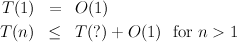
We can then attempt to write down a recurrence expressing the time requirements of the algorithms:
We have shown that the worst-case time required for search or insertion in a search tree is proportional to the number of nodes in the tree. This is not very impressive, since a similar performance could be obtained without using binary trees, by just using lists. The problem is that we have not put any constraints on the tree structure, so the function s(n) is bad. In an ideal world, we would like to have a perfectly balanced tree with s(n) = (n - 1)∕2, which would lead to T(n) = O(lg n). Unfortunately, the world of algorithms and data structures is not ideal, and we need to investigate compromise solutions, such as developing new strains of tree or allowing slightly less than perfect balancing of trees. Associated with these solutions are rather more complex sub-algorithms for insertion and deletion of elements, and we must ensure that these sub-algorithms do not themselves become too inefficient.
We shall now examine two possible ways to improve the structure of the trees used to implement dictionaries. One method involves a more complicated type of tree, and the other involves a slightly more flexible notion of balancing. It can be shown that the new tree types both have O(lg n) height, where n is the number of nodes. This will allow us to deduce that our algorithms require O(lg n) time.
An AVL tree (named after its inventors, Adel’son-Vel’skiĭ and Landis) is either:
with the additional property that a node’s two child sub-trees differ in height by at most one. This property, which we investigated in Practical 1, guarantees enough balance to support efficient dictionary operations. recall that an AVL tree of height h has at least fib(h + 2) internal nodes. So the height of the tree is O(lg n) where n is the number of nodes.
To represent an AVL tree, we shall store items at the nodes of a binary tree, as with simple binary search trees. Additionally, at each node, the difference in height of its two child sub-trees is recorded. We introduce a type Balance, with three values, L (the left subtree is higher); B, (the node is balanced, and the subtrees have the same height); and R (the right subtree is higher.
The sub-algorithm for searching is the same as the binary search tree sub-algorithm.
The sub-algorithm for insertion is rather more subtle. Its structure is the same as that for the binary search tree but, when a new node is created, it is necessary to ensure that the tree retains the AVL balance property. When we insert or delete an item, the resulting tree may have the same height as the original, or the heights may differ by one. We introduce a datatype Change with two constructors, C (changed), and U (unchanged), to keep track of this information. Without loss of generality, suppose that a new node is to be inserted into the left child sub-tree of a node. If the node’s left and right child sub-trees have the same height, there is no problem since the height of the left child is allowed to increase by one. If the node’s left child sub-tree has height one less the the right child, again there is no problem since the heights of both children are allowed to become the same. However, if the node’s left child sub-tree already has height one more than the right child, the balance property may be violated and then restructuring is necessary. In all cases, the restructuring can be effected by a repositioning of the node, the root of its left child and, in some cases, also the root of the left child’s own right child.
So, the insertion algorithm calls a subsidiary balancing function
fun ins (e, Lf) = (C, Nd(Lf, (B, e), Lf))
| ins (e, Nd(lt, (b,v), rt)) = if e < v then balins(ins(e, lt), (b,v), (N, rt)) else if v < e then balins((N, lt), (b,v), ins(e, rt)) else raise NoChange |
We give only one half of the definition of the balancing function, dealing with the case when the left-subtree of a node has grown. The other half can be obtained by symmetry. Note that even though there are many clauses, the necessary tree adjustments can be regarded as ‘simple things’, in the sense that they take O(1) time. This means that the insertion sub-algorithm’s behaviour can be analysed in the way outlined on the first page of this note.
fun balins((N, lt), v, (N, rt)) = (N, Nd(lt, v, rt))
| balins((C, lt), (L, c), (N, rt)) = let val Nd(t1, (ab, a), t2) = lt in case ab of L => (N, Nd( t1, (B, a), Nd( t2, (B, c), rt))) | B => (N, Nd( t1, (R, a), Nd( t2, (L, c), rt))) | R => let val Nd( t2, (bb, b), t3) = t2 val (bl, bn, br) = case bb of L => (B, B, R) | B => (B, B, B) | R => (L, B, B) in (N, Nd(Nd(t1, (bl, a), t2), (bn, b), Nd(t3, (br, c), rt))) end end | balins((C, lt), (B, e), (N, rt)) = (C, Nd(lt, (L, e), rt)) | balins((C, lt), (R, e), (N, rt)) = (N, Nd(lt, (B, e), rt)) | balins((C,_),_,(C,_)) = raise AVL |
There are many other ways to achieve adequate rough balancing of binary search trees. For example, red-black trees have the property that no path from a node to a descendant leaf has length more than twice that of a path from that node to any other descendant leaf. This is enough to ensure that the tree has O(lg n) height.
A 2-3 tree is either:
with the additional property that a node’s two or three child sub-trees have the same height. This property guarantees the balance required to support efficient dictionary operations.
To represent a dictionary using a 2-3 tree, we shall store items at the leaves, ordered from the smallest key at the leftmost leaf to the largest key at the rightmost leaf. At each node, the largest key in the first (left) child sub-tree and the largest key in the second (right or middle) child sub-tree are recorded. The sub-algorithm for searching is a simple variant of the binary search tree sub-algorithm already seen.
The sub-algorithm for insertion is rather more subtle. To insert a new item with key k, it searches down the tree until reaching the node that should have a leaf containing k as its child. If this node only has two children, a new leaf is added as an appropriately-positioned third child. If the node already has three children, things are not so simple, since it now needs four, which is illegal. In this case, the node is split into two parent nodes, one taking the two smallest children and the other taking the two largest children. Now, the problem is that the extra node needs to be added as a child of the original node’s parent. However, this is exactly the same as the problem of adding the new leaf, and so it is possible to proceed in a recursive manner while retracing the path followed by the initial search through the tree. If this recursion continues all of the way up the tree, and the root node is split into two, it is necessary to create a new root with the two nodes as its children; this is how the tree grows in height. In addition to any tree surgery, the ‘largest key’ records in all of the nodes traversed between the root and the leaf must be adjusted as necessary.
The insertion sub-algorithm produces a valid 2-3 tree with the new item added. Also, it should be clear that it involves a single sweep from root to leaf with a little work en route, followed by a return back from leaf to root with a little more work en route. Noting that a 2-3 tree of height h has at least 2h leaves, we can deduce that a 2-3 tree with n leaves has at most lg n height. Thus, the insertion and searching sub-algorithms both require O(lg n) time. [Exercise: devise a similar style of sub-algorithm for deleting an item in O(lg n) time.]
The idea behind 2-3 trees can be generalised to give B-trees. A B-tree of type t ≥ 2 allows a node to have between t and 2t children (e.g., the case t = 2 gives a ‘2-3-4-tree’). For large values of t, B-trees can be useful if data is kept on secondary storage rather than in primary memory. Since B-trees have O(lg n) height, they can be used to implement (large) dictionaries efficiently.
(C) Michael Fourman 1994-2006