1 Equational Reasoning

Our reasoning about ML programs will be based on the principle of replacing equals by equals — known grandiosely as equational reasoning. This is just the procedure familiar from algebra: we have general equations, which we use to simplify an expression. Here is an algebraic example:

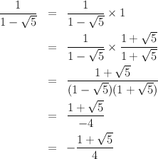
The key equation we use here is, (x-y)(x + y) = x² -y², but we use many other simpler facts, such as = 1. Notice that we apply specific instances of these general rules to replace part of an expression by something equal. This may seem laborious, but even here we have amalgamated some small steps.

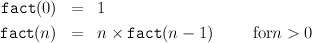
We will use the same kind of reasoning to deduce properties of our programs. Some of the general equations we apply come from mathematics; others come from the programs themselves. Consider the familiar factorial function:

fun fact 0 = 1     | fact n = n * fact (n-1)

Computing fact(n), for any n ≥ 0 yields a unique result, which can be arrived at by successively applying the equations

We can treat fact as a mathematical function, and use these equations to reason about it. Some of the equations have conditions attached, for example, the second equation for fact only applies when n > 0; this also occurs in algebra, for example, doesn’t make much sense when x = 0.

2 Proving Properties of Functions using Induction

Mathematical induction is used to prove that a property φ(n) holds for all natural numbers n. We prove that the base case holds, namely φ(0) is true. We then prove that φ(k) implies φ(k + 1) for all k. This is known as the inductive step. If we can prove both of these then we deduce, by induction, that φ(n) is true for all n. The induction rule can be written, more formally, as

The inductive step often looks as if we are cheating. However, we can use the inductive step to construct an explicit proof, for any given n. Suppose, for example, we want a proof that φ(5) is true. We know that φ(0) is true from the base case. We can then apply our inductive proof step for the case where k = 0 to get a proof that φ(1) holds. Applying the inductive step again, this time with k = 1, gives us a proof that φ(2) holds. We can obviously repeat this process until we get a proof of φ(5). This procedure is general: we can expand out the inductive proof to produce a non-inductive proof of φ(n) for any given n.

Often, to show φ(n), we must assume that φ(m), for some m that is smaller than n, but not necessarily exactly one smaller. A little thought should convince you that our justification of induction still works if we replace the inductive step by a proof that φ(k) holds under the assumption that φ(m) is true for all m < k. Indeed, if we can show this we don’t need an explicit base case; instantiating k to 0 gives a proof of φ(0) under the assumption that φ(m) is true for all m < 0. Since there are no natural numbers less than zero, the “inductive case” already includes a proof that φ(0). We refer to this variant of mathematical induction as complete induction. More formally,

We now demonstrate the use of complete induction on an ML example. Consider the function fastpower:

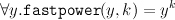
fun fastpower(x, 0) = 1     | fastpower(x, k) = if k mod 2 = 0 then fastpower(x*x, k div 2)                                        else fastpower(x*x, k div 2) * k

We show that for every natural number k,

Since the recursive call breaks down the problem by dividing k by two, the simple form of mathematical induction isn’t directly applicable in this case. However, for all k > 0, it is the case that (k div 2) < k, so we can use complete induction. Although we are using complete induction, we consider the cases k = 0, and k > 0 separately, because they are treated differently in the function definition.

In case k = 0, we must prove that fastpower(y, 0)  =  y⁰. But, y⁰  =  1 and fastpower(x, 0) returns 1; so substituting equals for equals does the job.

Now consider the case where k > 0. There are two sub-cases depending on whether k is even, i.e. kmod 2 = 0, or odd.

1. Suppose kmod 2 = 0, and kdiv 2 = j. So, k = 2j, and j < k. Now fastpower(x,k) = fastpower(x²,j), by the definition of fastpower. As j < k, the induction hypothesis allows us to assume that the conclusion, ∀y.fastpower(y,j) = y^j, holds; in particular, fastpower(x²,j)  =  (x²)^j. Putting these steps together with a little algebra, we have as required.
2. The case where k is odd is similar. We leave it as an exercise for the reader.

The fastpower function has two parameters; the second of these always gets smaller on each recursive call. This allowed us to perform an induction based on the size of this argument. The induction hypothesis includes all values of the other argument, this allows us to specialise it to the particular value used by the recursive call (in our example, x²).

Functions on products

Suppose that we want to verify the gcd function,

fun gcd(0,n) = n     | gcd(m,n) = gcd(n mod m, m)

We can use the approach given above, and show, by induction on m, that, for all n the result of evaluating gcd(m,n) is defined and is equal to the greatest common divisor of m and n. This general strategy applies as mrmmodn is always smaller than n.

Suppose instead that we wish to verify the following version of the gcd function, always assuming that it will only be applied to arguments greater than zero:

fun gcd(m,n) = if m = n then n                     else if m > n then gcd(m - n, n)                                   else gcd(m, n - m);

Note that in one of the recursive calls the first argument gets smaller and in the other call the second argument gets smaller. We can’t perform an inductive proof just based on the size of one of the arguments. Let’s look at the principle behind induction once again. We try to prove that a property φ holds assuming it holds for all smaller subproblems. As long as there isn’t an infinite sequence of smaller problems, then eventually we will encounter a subproblem for which we will have to prove φ without any assumptions. We can then use this to prove φ holds for the next larger problem, and so on, until we have a proof of the instance of the problem we are interested in.

So, the crucial property we are relying on is that there is an ordering on the problems such that the solution to a problem only relies on subproblems that are smaller in this ordering. Furthermore, the problems can’t keep on getting smaller and smaller indefinitely — we must hit the bottom eventually.

Technically, an ordering with this property is said to be well-founded. Complete induction can be used with any well-founded ordering, on any type. Clearly the ordering < on the natural numbers is well-founded; induction on natural numbers is a special case of this general principle.

For example, consider pairs of natural numbers. We can define a pair (a,b) to be smaller than (a′,b′) if max(a,b) < max(a′,b′). It is not difficult to see that this is a well-founded ordering on such pairs.

We now prove that our second implementation of gcd is correct using this ordering. In other words we prove that for any m > 0 and n > 0 the call gcd(m,n) returns the greatest common divisor of m and n, assuming that gcd(m’,n’) is true for all m’ and n’ such that the maximum of m’ and n’ is less than the maximum of m and n. We consider three separate cases:

1. Suppose m = n. Then gcd(m,n) returns n which is correct.
2. Suppose m > n. Then (m - n, n) < (m, n) and so we may assume that the call gcd(m - n,n) returns the gcd of m - n and n. Appealing to the properties of greatest common divisors, we can show that this is also the greatest common divisor of m and n.
3. Suppose n > m. The argument is symmetrical with the previous case.

3 Induction for Lists

We prove properties of ML functions on numbers, using induction on natural numbers and pairs of such numbers. Now we extend our techniques to allow us to reason about functions defined over lists. One approach is to perform induction based on the length of the list. An alternative is to develop an inductive strategy specifically aimed at reasoning about lists. We follow the second approach here, as it readily scales up to other datatypes.

Just as every natural number may be constructed from 0 by successively adding 1, so every list can be constructed from nil by successive applications of cons, ::. To prove a property φ(l) holds for all lists l it is sufficient to show

base case

that it holds for the empty list, nil, and

inductive step

if it holds for a list t, then it holds for all lists of the form h::t.

More formally, for any φ,

This is analogous to the definition of mathematical induction. Can you see what the analogue of complete induction would be in this case? The reason this technique is valid is analogous to the natural number case: we can use the base case and the inductive step to build a proof of φ(l), for any particular list, l, following the steps used to build the list from nil

In lazy functional languages, we can build infinite lists, in C we can build infinite lists by creating linked lists with cycles; it is much more difficult to give ,and apply, an inductive proof strategy covering such cases.

4 Induction for Trees

Trees are also built up inductively, so we can use inductive proof to show a property holds for all trees. Here, we consider binary trees, as introduced in Lecture Note 8; similar techniques apply to other varieties.

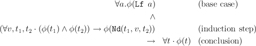
To prove that a property φ holds for all trees t it is sufficient to show

base case

that it holds for any leaf, Lf b, and

induction step

that, if it holds for t1 and t2, then it holds for all trees of the form Nd(t1,v,t2).

More formally, for any φ,

This technique is valid for the same reason as the other inductive techniques we have seen. Given any tree t, we can generate a non-inductive proof that φ(t) is true by starting with the empty tree and then using the inductive step to give us a proof of φ for larger and larger trees, until eventually we reach t.

We apply induction on trees to show the correctness of our efficient implementation of the function leaves, which lists the values at the leaves of a tree. Here are two function declarations

fun leaves (Lf a)        = [a]     | leaves (Nd(l, _, r)) = leaves l @ leaves r

and

fun accl(Lf a,        acc) = a :: acc     | accl(Nd(l, _, r), acc) = accl(l, accl(r, acc))

This definition follows a standard pattern: there are two parameters, a tree, and an accumulating parameter. The recursion is based on the structure of the tree parameter. This suggests a proof, by induction on the tree parameter, that some property holds for all values of the accumulator. We show, by induction on t, that,

Here is the proof

base case

induction step

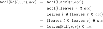
This may look more imposing than traditional algebra, but this is only because the rules are unfamiliar. To prove the base case, we use equations that come directly from the definitions of accl, @, and leaves. The induction step uses the definitions of accl and leaves, together with the associative law for append, which we leave as an exercise for the reader. ©Michael Fourman 1994-2006