Introduction

In Practical One, you will experiment with examples of SML functions — fac, fib, gcd and power. These are “obviously correct”; That is, the definitions of the functions are directly based on well-known mathematical relationships, and so we should have reasonable confidence in our programming efforts. The issue of correctness is of fundamental importance in software engineering, and will be addressed as the CS201 course progresses. However, in this note, we shall tend to take correctness for granted and worry instead about another important issue: efficiency.

Given some problem to be solved, we need to devise an algorithm, that is, a sequence of computational steps that transforms an input (i.e., a representation of a problem) into an appropriate output (i.e., a representation of the solution). When looking at the efficiency of algorithms, we are concerned with their resource requirements. In general, the two important resource measurements are the size of computer, and the amount of computer time, required by an implementation of an algorithm. For many problems, there are straightforwardly-expressed algorithms whose resource demands are sufficiently enormous that we need to find more subtle algorithms needing less resources. There is no guarantee that such algorithms will exist: usually it can be shown that problems cannot be solved using any less than some minimal level of resource.

Measuring resource requirements

If we have devised an algorithm, it possible to implement it by writing a computer program¹ and then to assess its efficiency by performing experiments. For example, for different inputs to the algorithm, we might measure the amount of memory space required, or the processor time required, to compute the outputs. Note that the latter measure is not usually the same as the actual time required, since the processor is likely to be doing other things as well as running the algorithm. You will have a little experience of experimentation in Practical One, where the time function will be used to measure the processor time required to evaluate various functions on various arguments. In some cases, this will yield unexpected observations worthy of further explanation.

The basic problems with an experimental approach to checking efficiency (and correctness, for that matter) are threefold. First, it is necessary to implement the algorithm: this may be time-consuming and error-prone. Second, details of the implementation may affect efficiency, and obscure the essential behaviour of the algorithm. Third, it is not normally possible to test the algorithm on all possible inputs, which may mean missing good or bad special cases.

Analysing resource requirements

As an alternative to experimentation, we shall be studying the analysis of algorithms as one thread of the course, that is, studying methods for predicting the resources that an algorithm requires. Analysing even simple algorithms can be challenging, and may require the use of non-trivial mathematics. The immediate goal of analyses is to find simple means of expressing the important characteristics of algorithms’ resource requirements, suppressing unnecessary details. Before embarking on an introduction to some of the technical tools required for analysis of algorithms, this note will review the algorithms from Practical One, to see what can be predicted about their resource requirements. To keep things simple, we shall restrict our attention to the computation time required, and not worry about memory space. In general, when writing down algorithms, we do not have to use a particular programming language, but can use an appropriate mix of notation and language that permits a rigorous description. For the algorithms here, SML descriptions are as good as any (and, of course, have the added advantage that they can be directly executed by a computer).

As Practical 1 will reveal, the basic problem with an analytic approach to predicting the performance of an algorithm is that we usually analyse a simplified computational model, which may abstract away features that, in practice, dominate the performance.

Analysis of factorial algorithm

The factorial algorithm can be expressed using simple recursion:

fun fact 0 = 1  
  | fact n = n * fact (n - 1);

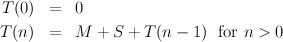
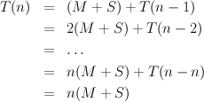
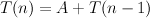
Looking at the computation that has to be done, we might identify three things that will consume time: integer multiplication, integer subtraction and recursive function calls. There are other possibilities but, if we try to take every little detail into account, we are unlikely to get any kind of simple analysis. Let us ignore the cost of making recursive calls, and suppose that the cost of a multiplication is M and that that of a subtraction is S. We can then define a function T(n), meaning “the time required by the algorithm to compute n!”, in a very similar form to that of the actual algorithm:

In this case, one obvious problem is an over-simplistic view of the cost of performing arithmetic. Regarding the subtraction time S as a constant is reasonable here, since n is a ‘normal size’ integer, i.e., fits into 16 or 32 bits, and so n-1 can be computed in one processor step. However, this is not the situation for multiplication. Employing some knowledge of the problem to be solved, we discover that n! grows very rapidly as n increases: Stirling’s approximation for the factorial function reveals that n! grows at roughly the same rate as nⁿ, so the number of bits needed to represent n! (that is lg n! where lg is the base-two logarithm function) grows at roughly the same rate as lg nⁿ = n lg n. Thus, it is not reasonable to charge a constant time for every multiplication: the number of bits used for the right-hand operand in n * fact (n-1) — roughly proportional to (n - 1) lg(n - 1) — will rapidly become larger than 16, 32 or whatever limit our processor has on normal integers.

Had we implemented the algorithm in C, we could not have used multiplication in such a cavalier fashion, since integers are not allowed to be bigger than the size that the processor can handle easily. To further understand our SML experiment, we need to establish how much time such a long multiplication takes, in terms of individual processor steps. Our SML system employs a straightforward algorithm (similar to long multiplication as learnt at school, in fact). This means that the time to multiply a normal size integer by a b-bit long integer is proportional to b. Thus, a more accurate expression for T(n) would be:

Analysis of Fibonacci algorithms

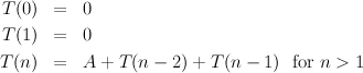
In the obvious Fibonacci algorithm, there are two conspicuous things that consume time: integer addition and recursive function calls. Letting A be a constant representing the time required for a simple addition, we can write down a function T(n) meaning “the time required by the algorithm to compute the n-th Fibonacci number”:

This is a very fast rate of growth, and helps to explain why our SML implementations run very slowly, even for modest values of n. The problem is the pair of recursive calls, which duplicate much work. A little thought leads to the alternative fastfib algorithm that eliminates one of the recursions, and so has:

(Highlights of) analysis of greatest common divisor algorithm

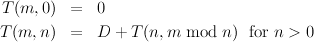
Letting D be a constant representing the time required for a division (needed to perform the mod operation), we can write down a function T(m,n) meaning “the time required by the algorithm to compute the greatest common divisor of m and n”:

(Exercise on) analysis of powering algorithms

Write down ‘time required’ functions for both the power and fastpower algorithms. You should be able to derive a non-recursive expression for the power time function fairly easily. [Hint: similar to the one for factorial.] Can you derive a non-recursive expression for the fastpower time function? (If not, await a lecture in the near future.) As with the factorial algorithm, we also have to think about the size of integers involved. When we do this, it turns out that there is not much difference between the performance of the two algorithms, as you may have discovered experimentally. With the SML implementation, there is a further twist: if the binary representations of intermediate values contain lots of zeroes (e.g., when computing powers of two), long multiplication is faster; this helps the fastpower algorithm.

Thus far, we have analysed various algorithms in a fairly informal way, starting from first principles each time. In the remainder of this note, we draw on our earlier experience in order to establish some general concepts that are useful whenever algorithms are being analysed and compared.

There are three main things to be introduced: standard simplifications to remove unnecessary detail from algorithms under consideration; some mathematical notation to express concisely the resource requirements of algorithms; and some algebraic techniques for manipulating formulae expressing resource requirements. We look briefly at the first two of these, and defer the algebraic techniques until later in the course.

Simplifying input detail

To quantify the resource requirements of an algorithm, we should really define a function that maps each possible input to a prediction of the algorithm’s resource requirement on that input. However, for all but the most trivial types of input, this is a daunting undertaking because of the number and variety of different inputs possible. Therefore, we normally distill the inputs to get a simpler characterisation: the input size. Usually, when viewed at a low enough level of abstraction, the size of a ‘reasonable’ binary representation of the input is a good measure. This allows some comparison of the resource requirements of algorithms from widely different problem areas. However, within specific problem areas, it is often clearer to define input size at an appropriate higher level.

The insertion of the word “reasonable” above is designed to avoid occasions where we appear to be solving large problems cheaply but where we are, in fact, solving small problems expensively, because the algorithm input is represented in a way far more complicated than necessary. As a rough guide to what is reasonable, we can be guided by a fundamental result from information theory: if a data type has k different values, each of which is equally likely to occur as inputs, then n lg k bits are necessary and sufficient to represent a sequence of n inputs. As an indication that this result is not unexpected, consider numbering the different values from 0 to k - 1, and recall that lg k bits are necessary and sufficient to represent these integers uniquely. (As an indication that the result is not trivial, observe that if some values occur more frequently than others we may transmit messages more efficiently by using a code with fewer bits for more frequent characters.)

After defining the input size measure for an algorithm, we define a function that maps each input size to a predicted resource requirement ‘on that input size’. The trouble is that there is usually a range of requirements: some inputs of a given size may be very cheap to deal with, others may be very expensive. Normally, we determine the requirements of the worst possible input of each size in order to characterise the behaviour of an algorithm. Sometimes however, where it is clear that an algorithm is normally far better than a worst case analysis suggests, we determine the average requirement over all the inputs of a given size. The analysis of the quick sort algorithm later in the course will give an example of this.

Simplifying computational detail

To predict the time required for the execution of an algorithm², we shall attempt to predict how many ‘elementary computational operations’ are performed. The working definition of “elementary” will be that an operation requires some constant amount of time to carry out, that is, the time does not vary with the size of the operands. Everyday examples include adding two 64-bit real numbers, comparing two 32-bit integers, or moving a 16-bit integer from one location to another. Outlawed examples include adding two arbitrary length integers, or searching an arbitrary-length list for an item of interest. To avoid our analyses becoming dependent on implementation details, we shall not exactly quantify the constant amounts of time required for elementary operations. This simplification still allows us to examine the basic behaviour of algorithms, and to compare alternative algorithms.

As the informal analyses given earlier may have suggested, we shall make a further abstraction to simplify matters: only the rate of growth of the time requirement with respect to increasing input size is of interest. Therefore, instead of aiming to derive a fairly precise formula to express an algorithm’s time requirements, e.g., T(n) = 10n² - 2n + 9 elementary operations where n is the input size, we shall only aim to establish the dominant highest order term, here 10n². Moreover, we shall ignore the constant coefficient, here 10, since constant factors are less significant than the rate of growth in determining efficiency for large input sizes. Given these simplifications, we can express formulae for resource requirements concisely using ‘big-O’ notation. The formula

there are two constants, c and n₀, such that

(we assume that none of c, n₀, T(n) or f(n) is ever negative). In the example above where T(n) = 10n² - 2n + 9, we just write T(n) = O(n²). Here, f(n) = n², and c = 10 and n ₀ = 5 are suitable constants. Note that T(n) does not have to grow as fast as f(n); saying T(n) = O(f(n)) merely asserts that T doesn’t grow any faster than f. Usually, the functions f(n) that we see are of the form n^k (where k is a constant), lg n or 2ⁿ, or some multiplicative combination of these, such as n² lg n or n2ⁿ. Note that lg n grows more slowly than any function of the form n^k, for every k > 0 —even when k < 1, and 2ⁿ grows more quickly than any function of the form n^k. One useful, and slightly abused, special case is f(n) = 1: the formula T(n) = O(1) is used as shorthand for “T(n) is bounded by some constant for all n”.

We usually consider that one algorithm is more efficient than another algorithm if its time requirement has a lower rate of growth. Note that may not be faster for some input sizes, but the algorithm will be faster for all large enough inputs. When comparing algorithms on the basis of big-O notation formulae, we must take care that the hidden n₀ thresholds and the hidden c constant factors are not outrageously large. Remember that, for example, a O(n) time algorithm requiring 1000000n operations is slower than an O(n²) one requiring n² operations unless n > 1000000.

Deriving formulae for time requirements

The examples given earlier should indicate that it may be fairly straightforward to derive a recursive definition for the time requirement of a given algorithm. Solving such definitions to obtain an algebraic formula for the complexity is sometimes a taxing mathematical challenge. However, many examples are straightforward, and different algorithms may often be treated using similar methods. We will return to look at some of these techniques later in the course. For the moment, as an exercise, we derive O-expressions for the rates of growth of the various recursively defined functions, counting nodes and leaves of trees, introduced in Lecture Note 1.

Full Trees

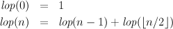
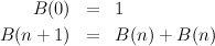
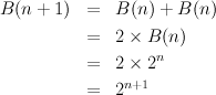
The number of leaves in a full binary tree of height n is given by the equations:

Spines

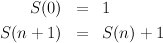
The equations for the number of leaves in a spine

Balanced trees

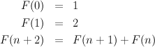
The number F(n) of leaves in a slightly unbalanced tree is given by the following equations:

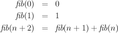
The Fibonacci numbers are related to the golden ratio, φ = , and its conjugate, = . These are defined as the roots of the quadratic equation φ² = 1 + φ. Numerically, φ = 1.61803…, and = -0.61803…. The ith Fibonacci number fib(i) is equal to (this may be proved by induction on i). Since | | is less than 1, the term ⁱ∕ is small, and φⁱ∕ is a good approximation to fib(i) (rounded to the nearest integer, it is equal to fib(i)). The upshot, for our present purposes, is that F(n) is also exponential.

Lop-sided trees The least number of leaves in a tree of height n, imbalanced at any node by at most a factor of 2, is given by the recurrence