Sorting and Searching

Michael P. Fourman

October 31, 2006

Introduction

There is an intimate relationship between algorithms and datastructures. Some algorithms depend on particular datastructures; more important, some ideas can be transferred from algorithms to the design of data structures, and vice-versa. One important method in computer science is to “divide and conquer”. This idea underlies the efficient implementation of sets and dictionaries using trees. In this note, we review some sorting algorithms that make effective use of the divide-and-conquer strategy.

When we examine algorithms for computing various functions over the integers, we attempt to derive simple formulae to express the amounts of computation time required. We try to derive an expression for the time required in terms of the algorithm input itself, e.g., that the time to compute n! is roughly proportional to n.

In general, this is not possible because the type of the input will be rather more complicated than just a single integer or a pair of integers. Such a difficulty occurs when we undertake an analysis of sorting algorithms. Nothing will be assumed about the type of the items, except that it must be possible to compare any pair to determine which item comes first in the ordering. Given this, rather than attempting to define ‘time required’ functions in terms of the fine detail of the collection of items supplied as input to a sorting algorithm, we shall define functions in terms of a much cruder, integer, measure: the number of items in the collection. This is adequate to allow basic analysis and comparison of various algorithms.

When studying sorting algorithms we consider comparing two items as a basic operation. A fundamental consideration is the number of comparisons between items an algorithm must make to sort a given collection. This is because all the sorting algorithms we consider proceed by performing a series of item comparisons, possibly adjusting the representation of the item collection after each comparison.

We fix on a type of Item to sort, equipped with a comparison operator <=, and consider the problem of sorting a list of items. We begin with some naive sorting algorithms.

Insertion sort

A sorting algorithm based on insertion is simple to describe: consider each item in turn, and insert it into its correct place amongst all of the items already considered. Such an algorithm is sometimes used by humans, for example card players sorting their hands into order. We can phrase the algorithm in simple recursive terms as just: insert one item from a collection into its correct place in the recursively-sorted remainder of the collection.

local fun insert i (h :: t) = if i <= h then i :: h :: t
                                       else h :: insert i t
        | insert i  []      = [i]
   in fun isort []       = []
        | isort (h :: t) = insert h (isort t)
end;

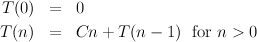
To assess the time required by the algorithm, we must first examine the insert sub-algorithm that inserts an item i into a sorted collection, of size n say. The number of comparisons ranges from one, if i goes first, to n, if i goes last. Adopting a pessimistic air, we shall assume the worst: insertion time is roughly proportional to n. Now, we can define a function T(n), meaning “the time required by the isort algorithm to sort n items, at worst”:

T(0) = 0 T (n) = Cn + T(n - 1) for n > 0

where C is a constant of proportionality big enough to cover the cost of insertion. From this,

T (n) = Cn + C(n - 1) + ...+ C + 0 = Cn(n + 1)∕2

and so the time required is roughly proportional to n². Remember that this is the worst case time for the algorithm — sometimes, for example if the collection is already sorted, the time is just roughly proportional to n. However, it is not hard to show that, for a ‘randomly ordered’ collection of n items, the expected time is, in fact, roughly proportional to n².

Bubble sort

The insertion sort algorithm has the merits of being easy to believe in, easy to implement and, for smallish collections of items, fast enough to be of practical use. It is less clear why the bubble sort algorithm has acquired such popularity in recreational computing circles since, compared with insertion sort, it is less easy to understand, harder to implement and usually slower. We include it here for completeness.

If a collection of items is not fully sorted, the bubble sub-algorithm ‘bubbles’ one or more items through the collection in order to improve its orderliness. The bsort algorithm invokes the sub-algorithm repeatedly until it does not change the ordering of the collection, which means that the collection must be completely sorted.

local fun bubble (h :: k :: t) = if h <= k then h :: (bubble (k :: t))
                                           else k :: (bubble (h :: t))
        | bubble x = x
   in fun bsort l = let val l’ = bubble l
                     in  if l’ = l then l else bsort l’
                    end
end;

The time required by the bubble sub-algorithm when applied to a collection of n items is roughly proportional to n, since n- 1 comparisons are performed. The time required by the bsort algorithm to sort a collection of n items depends on how much bubbling is required, ranging from one bubble, if the collection is already sorted, to n bubbles, if the collection is originally in reverse order for example. It can be shown that for a ‘randomly ordered’ collection of n items, the expected number of bubbles is roughly proportional to n. Thus, in the worst case and also on average, the time required by the bsort algorithm is roughly proportional to n × n = n², as it was for the insertion sort algorithm.

The complexity of these linear processes for sorting is O(n²). This is because in each case we step through the n elements, and for each element perform two operations (select and insert) one of which is trivial (and takes constant time), while the other can take O(n) time. To improve on this complexity, we must use a more subtle pattern of computation.

Selection sort

Selection sort is the dual of insertion sort. Whereas insertion sort selects a random element (in fact, the first) and carefully inserts it in the right place in the sorted list, selection sort carefully selects the smallest element, and then places it at the beginning of the sorted list.

local
   fun getMin [a] = (a,[])
     | getMin (h :: t) = let val (m, t’) = getMin t
                         in
                             if h <= m then (h, t)
                                       else (m, h :: t’)
                         end
in
   fun ssort [] = []
     | ssort x  = let val (m, t) = getMin x in m :: ssort t end
end

The work is the same: getMin must traverse the remaining list each time it is called—and it is called for each element. So we again make n² comparisons.

Divide and Conquer

There is a saying that, ‘a problem shared is a problem halved’. This is true!. Suppose we have an O(n²) algorithm for sorting, then to sort 100 objects may take four times as long as sorting 50 objects; if we divide our 100 objects into two lots of 50, then we can sort both of these in half the time. A problem shared is indeed a problem halved — even when we consider the work of solving both halves. Of course we still have to combine the two solutions, but we can merge the two sorted lists together in a single pass O(n) time. This idea is the basis of mergesort: to sort a list, divide it in two, sort the two halves and merge the results. What algorithm should we use to sort the two halves? — Use mergesort again. Isn’t this circular? — Not quite; some lists are so small that sorting them is trivial — for these we won’t need to use mergesort again.

Mergesort

local
    fun divide (a :: b :: rest) =
        let val (x,y) = divide rest in (a :: x, b :: y) end
    |   divide x = (x, []) ;

    fun merge (a :: x) (b :: y) =
        if a <= b then a :: merge x (b :: y)
        else b :: merge (a :: x) y
    |   merge x [] = x
    |   merge [] y = y ;
in
    fun msort (a :: b :: z) =
        let val(x,y) = divide (a :: b :: z)
        in merge(msort x) (msort y) end
      | msort x = x
end

An analysis of mergesort must consider the pattern of recursive calls. These form a binary tree; each non-terminating call makes two recursive calls (to sort lists of half the length). In merging two lists we remove one item for each comparison we make, so the number of comparisons made at each level of the tree is at most one for each element of the original list. The tree has O(lgn) levels, so the total number of comparisons is O(nlgn).

Quick sort

In merge sort all the sorting is done as we merge the lists together. The function that divides them up doesn’t even need to know what the ordering is. This is reminiscent of insertion sort, where the selection function was trivial and the insertion function did the work. We now consider another divide-and-conquer sorting algorithm, related to merge sort just as selection sort is to insertion sort. The idea is to divide the list into two parts such that if we sort them, then ‘merge’ them trivially by placing one after the other, we will sort the whole list. Clearly, we must divide the original list into two so that all elements in one part are greater than or equal to all elements in the other.

local
    fun divide x (h :: t) =
        let val (low, high) = divide x t
        in if x < h then (low, h :: high)
                     else (h :: low, high)
        end
      | divide _ [] = ([],[])

    fun merge x (a, b) = a @ [x] @ b
in
    fun qsort (h :: t) = let val (x, y) = divide h t
                         in merge h (qsort x, qsort y)
                         end
      | qsort [] = []
end ;

Quicksort comes right after Euclid’s Algorithm in the List of Famous Algorithms, partly because it is brilliantly named, but primarily because it usually lives up to its name. It is efficiently implementable in place using a fixed array to store the various subproblems generated in the course of the algorithm. The analysis of quick sort is similar to that of merge sort, except that divide is now non-trivial, and cannot be relied on to split the problem evenly in two. In some cases, the algorithm will only split off one element from the rest. If this happens repeatedly, the depth of the tree representing the computation is n - 1. We still have to process n elements at each level, so, the worst case complexity is O(n²). Nevertheless, for randomly ordered inputs, you can expect quicksort to take O(nlgn) time.

The implementation given above is wasteful; the repeated use of append is unnecessary. Much earlier, we used an accumulating parameter to eliminate append from our tree traversal algorithms. We can use that idea again here.

local
    fun divide x (h :: t) =
        let val (low, high) = divide x t
        in if x < h then (low, h :: high)
                     else (h :: low, high)
        end
      | divide _ [] = ([],[])

    fun qs (h :: t)  a = let val (x, y) = divide h t
                         in qs x (h :: qs y a)
                         end
      | qs [] a = a
in
    fun  qsort x = qs x []
end ;

O’Keefe’s algorithm

In our analysis of mergesort, and quicksort we only considered the number of comparisons made by the algorithms. In fact they both spend a great deal of time in list manipulations. This does not affect the asymptotic complexity of the algorithms; a detailed analysis of the list manipulations is similar to the one we’ve sketched for counting comparisons. Nevertheless, for practical implementations it is worthwhile to eliminate some unnecessary work.

O’Keefe applied an idea similar to Vuillemin’s heaps to give a more efficient implementation of mergesort. We want to ensure that we always merge two lists of similar size. We maintain a list of lists, ensuring that the list in the i^th place is either empty (a “zero”) or contains 2ⁿ elements (a “one”). We add elements to the data-structure by propagating a carry from the least-significant “digit”. When we propagate a carry we merge two lists of size 2ⁱ to get a list of size 2ⁱ⁺¹. Finally, we merge the resulting list of lists, to “flatten” the data-structure to a single list.

O’Keefe’s algorithm takes this idea one stage further. The input to a sorting routine may contain runs of elements that are in order. Rather than split a run up into singleton lists, and then re-merge them we can carry the entire run into our data-structure. The sizes of the lists are no longer powers of two, but the number of merge operations used to build a list in the i^th place is still i.

local
    fun merge (a :: x) (b :: y) =
        if a < b then a :: merge x (b :: y)
        else b :: merge (a :: x) y
    |   merge x [] = x
    |   merge [] y = y ;

    fun carry []     x     = x
      | carry x      []    = [x]
      | carry x ([] :: aa) =  x :: aa
      | carry x  (a :: aa) = [] :: carry (merge x a) aa

    fun flatten []  = []
      | flatten [h] = h
      | flatten (h :: k :: t) = flatten(merge h k :: t)

    fun revs [] a = a
      | revs (h :: t) a = revs t (h :: a)

    fun runup(up, x :: y :: t) =
        if x < y then runup(revs up [x], y :: t)
                 else (x :: up, y :: t)
      | runup(up, xs) = (revs up xs, [])

    fun rundown(down, x :: y :: t) =
        if y < x then rundown(x :: down, y :: t)
                 else (x :: down, y :: t)
      | rundown(down, xs) = (xs @ down, [])

    fun sorting (x :: y :: t) =
        let val (h, t) = (if x < y then runup else rundown) ([x], y :: t)
        in carry h (sorting t) end
      | sorting x = [x]
in
    fun oksort x = flatten (sorting x)
end

Appendix

Debugging ML programs

By far the easiest, and best, way to avoid bugs is not to introduce them in the first place. Write code in small chunks. Have a clear understanding of the type of each function you write; use the compiler to check your understanding. Use PolyML.ifunctor to help you write interactively. Test each function interactively where possible.

Pay attention to compiler warnings. They may highlight “typos” or misunderstandings. Match or Bind exceptions at run-time may result if you ignore warnings.

Finally, you may need help tracking down run-time errors, or help understanding the behaviour of your code. The compiler provides some tools to assist you.

The function PolyML.print : ’a -> ’a returns the value passed to it unchanged, but also prints a representation of the value to the screen. It can help you inspect values that are passed as parameters within your code. The compiler must be able to deduce the type of the value at compile time, in order to produce a meaningful representation.

The function PolyML.exception_trace : unit -> ’a -> ’a takes a suspension as argument and evaluates it. If this evaluation raises an un-trapped exception, a trace of the function calls leading up to the error is printed to the screen. For example, if evaluation of (f x) raises an exception, it may be helpful to execute
PolyML.exception_trace( fn () => f x );
to see what sequence of calls led to the exception.

Release Procedures

It is not a good idea to keep changing code right up to the deadline. Last minute changes introduce errors more often than they eliminate them. In industry code is usually “frozen” some time before the release date (a month, or more, is common). You don’t have the luxury of a month of slack in the schedule; however, you should aim to complete your changes well in advance of the deadline, and use the remaining time to tidy up and test your code so that you can explain its behaviour during the demonstration. Prepare a list of known bugs and bring it with you to the demonstration.