In the case of recognition a reasonable strategy is to maintain a list of plausible hypotheses and accumulate evidence for each one through a sequence of observations, which we refer to as temporal regularization (Another example of a sequential strategy can be found in [7].). We will show how this can be precisely formulated in probabilistic terms using Bayesian chaining strategy to effect regularization. The hope is that experimental results will confirm the validity of the general position assumption by showing that in most cases the list of plausible hypotheses quickly diminishes to a single confident assertion.
The foregoing begs the important question of whether it is possible to create an appearance manifold for sufficiently general motions in the first place. Clearly this is possible in restricted contexts such as gesture recognition. What we seek is a means of generating a set of canonical motions, i.e. a motion basis, in different viewpoints that can generalize to a sufficiently wide range of appearances to be of use in practical recognition tasks. Again, we invoke a second general assumption regarding the motion of physical objects:
This suggests that a motion basis can be constructed by presenting an object to a stationary observer and sweeping it in different directions in the plane tangent to the current viewing direction. The basis is constructed be repeating this process for each of the object's canonical viewpoints. (Equivalent motions can be induced by moving the camera about a stationary observer.) Additionally we need to assume that the object moves at constant velocity relative to the camera, which is in general not a severe constraint. In the next section, we discuss precisely how this appearance manifold can be built.
Building an appearance flow manifold
Flows corresponding to the expected motions of a mobile object moving about a stationary observer are induced during training by moving the observer (a television camera) on a tessellated viewsphere surrounding the object of interest according to the the following set of constraints:- Camera Constraints. Camera to object distances are bounded and scaled orthographic projection is assumed.
- Motion Constraints. The same motion model can be used to account for an object moving about a fixed observer and vice-versa provided that rotations are limited to axes that are approximately parallel to the image plane.
- Motion Decomposition.Assumption A2 applies equally to the case of the mobile observer.
Constraint 1 is required to ensure that a sufficient component of the optical flow magnitude is due to the structure of the object. Together with Constraint 2, it then becomes possible to associate the magnitude of the optical flow vector with distance to the camera. Taken as a whole, the magnitude of the optical flow field can be viewed as a rough kinetic depth map. This is by no means adequate for quantitative recovery of structure due, among other things, to confounding with motion, but it can provide a basis for recognition according to general position assumption A1. Constraint 3 implies that the structure component induced by camera motion about a stationary object is indistinguishable locally from that induced by the motion of the object about a stationary observer. This permits the construction of a motion basis using the more tractable approach of a mobile observer moving about a stationary object. The question of how to generate this basis from sensor motion is discussed next.
By assuming that objects can be differentiated on the basis of their local structure over time, the range of motions that needs to be generated during training is reduced significantly (Assumption A2). However this range is still considerable encompassing 4 degrees of freedom: viewsphere position, direction of motion (component parallel to the plane tangent to the surface), height above the surface, and curvature of the arc (direction orthogonal to surface). Prior knowledge about how objects are likely to interact with the observer can be used to further restrict the range of motions that need to be sampled. For example, the object can be kept at a fixed canonical pose with respect to the camera (i.e. the camera was kept upright) during the acquisition of training images. Each object is then sampled using only 184 trajectories corresponding to 2 orthogonal sweeps at a fixed distance from the object with the same radius of curvature as the surrounding viewsphere at each of 92 viewsphere directions. Experimental results would be required to show that this basis is sufficient to generalize to a very broad range of novel motions.
Each of the 184 trajectories gives rise to a distinct motion sequence,
si,j,t, where the indices i,j, and
t are used to reference a particular object, trajectory, and image
within the sequence respectively. Figure 1 shows a sequence of 1
images resulting from motion in a vertical arc on a viewsphere
surrounding one of the test objects (a horizontal arc can be seen as well).
An optical flow algorithm is used to estimate for each
si,j,t, t=1..l, a vector field,
vi,j,t,t=2..l-1, corresponding to the optical flow
field induced by the camera motion. Only the magnitudes of
vi,j,t are of interest here (for the reasons cited
earlier). For the particular optical flow algorithm chosen [15], three images
were required to estimate a single optical flow vector. As three samples along
each trajectory were sufficient to characterize each curvilinear sweep, each
object i gives rise to a set of 184 scalar images. For brevity we
refer to the latter as flow images. Standard PCA (principal component
analysis) techniques [1] are used to construct an eigenbasis for the entire
training set of 4600 flow images.
Let each of these images be represented by an m x n x 1 vector, dj, with m and n corresponding to the image dimensions. We refer to the latter as an image flow vector. A representation for each object is subsequently constructed by projecting each of its corresponding N image flow vectors dj|j=1..N onto the eigenbasis and representing the resulting set with an appropriate parameterization. We refer to the latter as the appearance flow manifold. For the experiments presented in this paper, the manifold is parameterized with a multivariate normal distribution of the form N(mumi,CTi), where the sample mean, mumi, and sample covariance CTi, are estimated in the usual manner.
Sequential recognition strategy
On-line, a sequence of images is gathered by moving an unknown object in front of the camera via a set of curvilinear movements. Let d correspond to a single image flow vector computed from this sequence. The first step in the recognition process is to compute the support for each object hypothesis, Oi, i=1..K, i.e. the probability that the single image flow vector, d, corresponds to each object, represented by p(Oi|d). Using standard Bayesian techniques leads to the following solution for each p(Oi|d) [16,17]:
where p(Oi) is the prior probability of object hypothesis i, and N(mumi,CTi) |m=m(d) is the multivariate normal distribution representation for the object hypothesis, evaluated at the projected parameters of the measurement, m=m(d).
As each of the image flow vectors is computed from a set of intensity images, evidence can be inexpensively and efficiently accumulated on the level of the probabilities over time, by using a Bayesian chaining strategy that assigns the posterior probability distribution at time t, p(O|dt), as the prior at time t+1. In this fashion, probabilistic evidence is cascaded until a clear winner emerges. Substituting the posterior density function derived from one view (derived in the previous equation) as the prior for the next view leads to the following updating function for p(O|d) [16,17]:
The hypothesis is that confounding information in the optical flow signatures
can be resolved by accumulating support for different object hypotheses over a
sequence of observations in this manner according to Assumption A1.
Presenting the system with all prior evidence should resolve ambiguities and
lead to a winning solution in a short number of views. The entire system can
be seen in Figure 2.
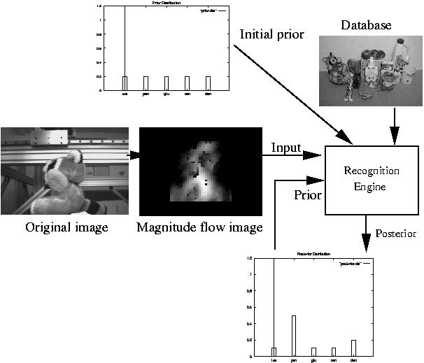
Figure 2: As each flow image in the sequence is introduced to the system, probabilistic evidence is cascaded until a clear winner emerges. The idea is that strong prior evidence should resolve ambiguities and lead to a winning solution in a short number of views.
The next task is to determine a suitable convergence criterion for the
system. It can be shown that a metric that predicts the likelihood of
ambiguous recognition results as a function of the measurement can be derived
based on Shannon's entropy [18]:
which is a measure of the ambiguity of the posterior distribution produced by a recognition experiment. Higher entropies reflect greater ambiguity. Using this metric, the system is said to converge when it reaches some on-line entropy threshold, set to some arbitrarily low value.
Experiments
To test this hypothesis we have constructed in our laboratory a robot-mounted
camera system that can generate the requisite sensor trajectories on a
viewsphere surrounding the object of interest. This apparatus is used to
automatically generate motion bases (training) for a set of approximately 25
standard household objects. On-line, objects from the database are presented
to a stationary camera by subjecting each to a set of curvilinear motions
generated by a precessing pendulum (using the object as the mass). This
approach allows for a wide range of sample trajectories that are clearly
outside of the motion basis used for training (see Figure 4).
In addition, we have also
performed testing on free rotations and translations generated by hand.
Figure 4: Setup consists of a person swinging an object in front of a stationary camera.
Through application of the sequential recognition strategy, the system is shown to converge to a correct assertion in terms of its MAP (maximum a posteriori ) solution in the majority of cases. This lends support to our contentions regarding the generalizability of our motion basis and disambiguation of competing hypotheses via temporal regularization. Figure 5 plots the entropy over time for the case of a panda bear moved in front of the camera. The system starts with an incorrect assessment about the object identity. Notice that as the object continues to swing in front of the camera, the system becomes more certain about its identity. In time, it converges to the correct solution.
Figure 5: On-line entropy of recognition results over time for panda bear. The MAP solution is shown above the curve at each iteration.
References
- M. Turk and A. P. Pentland, "Face Recognition Using Eigenfaces", in Proceedings of the International Conference on Computer Vision, 1991, pp. 586-591.
- S. K. Nayar, H. Murase, and S. A. Nene, Parametric Appearance Representation in Early Visual Learning, chapter 6, Oxford University Press, February 1996.
- T. Jebara, K. Russell, and A. Pentland, "Mixtures of eigenfeatures for real-time structure from texture", in Proceedings of the 6TH International Conference on Computer Vision, Bombay, India , IEEE Computer Society Press, Jan 1998.
- M. Kirby and L. Sirovich, "Application of the karhunen-loeve procedure for the characterization of human faces", IEEE Transactions on Pattern Analysis and Machine Intelligence, vol. 12, no. 1, 1990.
- W. Wahid B. Moghaddam and A. Pentland, "Beyond eigenfaces: Probabilistic matching for face recognition", Tech. Report 443, M.I.T. Media Laboratory Perceptual Computing Section, 1998, Appears in: The 3rd IEEE Intl. Conference on Automatic Face and Gesture Recogntion, Nara, Japan, April 1998.
- L. Sirovich and M. Kirby, "Low-dimensional procedure for the characterization of human faces", Journal of the Optical Society of America, 4:3, 1987, pp. 519-524.
- N. Li, S. Dettmer, and M. Shah, "Visually recognizing speech using eigen sequences", MBR97, 1997, Chapter 15. \bibitem{Pentland:96}
- A. Pentland, R. W. Picard, and S. Sclaroff, "Photobook: Content-based manipulation of image databases", International Journal of Computer Vision, 18:3, 1996, pp. 233-254.
- R. Campbell and P. Flynn, "Eigenshapes for 3d object recognition in range data", in Proceedings of the IEEE Computer Society Conference on Computer Vision and Pattern Recognition, Fort Collins, CO, vol. 2, IEEE Computer Society Press, June 23-25 1999, pp. 505-510.
- N. T. M. Watanabe and K. Onoguchi, "A moving object recognition method by optical flow analysis" In Proceedings of the 13th International Conference on Pattern Recognition, volume 1 of A, pages 528-533, Vienna, Austria, Aug 1996. International Association for Pattern Recognition.
- A. F. Bobick and J.W. Davis, "An appearance-based representation of action", Technical Report 369, MIT Media Lab, February 1996. As submitted to ICPR 96.
- M. J. Black and Y. Yacoob, "Recognizing facial expressions in image sequences using local parametrized models of image motion", Int. Journal of Computer Vision, 25(1):23-48, 1997. Also found in Xerox PARC, Techinical Report SPL-95-020.
- T. J. Darrell and A. P. Pentland, "Recognition of space-time gestures using a distributed representation", Technical Report 197, M.I.T. Media Laboratory Vision and Modelling Group, 1992.
- S. Vinther and R. Cipolla, "Active 3d object recognition using 3d affine invariants" In J.-O. Eklundh, editor, In Proc. 3rd European Conf. on Computer Vision, volume II of LNCS 801,, pages 15-24, Stockholm, Sweden, May 1994. Springer-Verlag.
- S. M. Benoit and F. P. Ferrie, "Monocular optical flow for real-time vision systems", In Proceedings of the 13th International Conference on Pattern Recognition, pages 864-868, Vienna, Austria, 25-30, Aug. 1996.
- T. Arbel and F. P. Ferrie, "Viewpoint Selection by Navigation through Entropy Maps", in Proceedings of the Seventh IEEE International Conference on Computer Vision, Kerkyra, Greece, Sept 20-25, 1999, pp. 248-254.
- T. Arbel and F. P. Ferrie, "Recognizing Objects by Accumulating Evidence Over Time", in Proceedings of the Fourth Asian Conference on Computer Vision, Taipei, Taiwan, Jan 8-11, 2000, pp. 437-442.
- T. M. Cover and J. A. Thomas, Elements of Information Theory, Wiley and Sons, New York, 1991.
A presentation on this topic was given at the Eleventh British Machine Vision Conference, Bristol, UK, 11-14 September 2000. Download the paper.