To understand kernel estimators we first need to understand histograms whose disadvantages provides the motivation for kernel estimators. When we construct a histogram, we need to consider the width of the bins ( equal sub-intervals in which the whole data interval is divided) and the end points of the bins (where each of the bins start). As a result, the problems with histograms are that they are not smooth, depend on the width of the bins and the end points of the bins. We can alleviate these problem by using kernel density estimators.
To remove the dependence on the end points of the bins, kernel estimators centre a kernel function at each data point. And if we use a smooth kernel function for our building block, then we will have a smooth density estimate. This way we have eliminated two of the problems associated with histograms. The problem of bin-width still remains which is tackled using a technique discussed later on.
More formally, Kernel estimators smooth out the contribution of each
observed data point over a local neighbourhood of that data point.
The contribution of data point x(i) to the estimate at some point
x![]() depends on how apart x(i) and x
depends on how apart x(i) and x![]() are. The extent of this contribution is dependent upon the shape of
the kernel function adopted and the width (bandwidth) accorded to
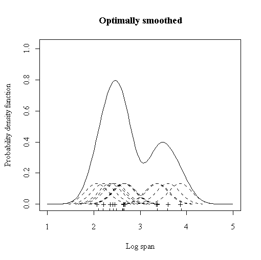
it. If we denote the kernel function as K and its bandwidth by
h, the estimated density at any point x is
are. The extent of this contribution is dependent upon the shape of
the kernel function adopted and the width (bandwidth) accorded to
it. If we denote the kernel function as K and its bandwidth by
h, the estimated density at any point x is
where ![]() to ensure that the estimates f(x) integrates
to 1 and where the kernel function K is usually chosen to be
a smooth unimodal function with a peak at 0. Even though Gaussian
kernels are the most often used, there are various choices among kernels
as shown in the table below.
to ensure that the estimates f(x) integrates
to 1 and where the kernel function K is usually chosen to be
a smooth unimodal function with a peak at 0. Even though Gaussian
kernels are the most often used, there are various choices among kernels
as shown in the table below.
| Kernel | K(u) |
| Uniform |
|
| Triangle |
|
| Epanechnikov |
|
| Quartic |
|
| Triweight |
|
| Gaussian |
|
| Cosinus |
|
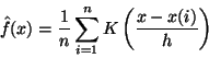
The quality of a kernel estimate depends less on the shape of the K than on the value of its bandwidth h. It's important to choose the most appropriate bandwidth as a value that is too small or too large is not useful. Small values of h lead to very spiky estimates (not much smoothing) while larger h values lead to oversmoothing. The following three figures (http://www.maths.uwa.edu.au/ duongt/seminars/intro2kde/) show the effect of 3 different bandwidths. When the bandwidth is 0.1 (very narrow) then the kernel density estimate is said to undersmoothed as the bandwidth is too small.
 |
 |
 |
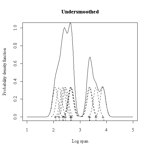
We can try to alleviate it by increasing the bandwidth of the kernel to a larger value (0.5). But, now we obtain a much flatter estimate with only one mode in place of the earlier four. This situation is said to be oversmoothed as we have chosen a bandwidth that is too large and have obscured most of the structure of the data.
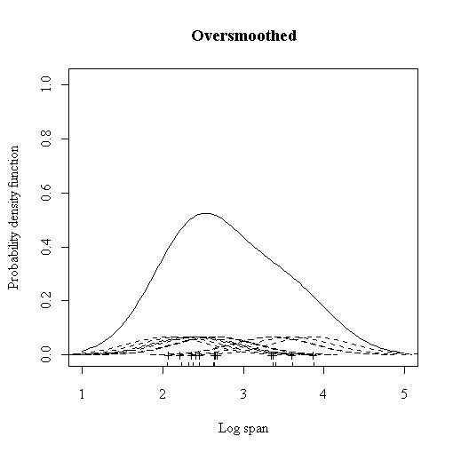
A common method to choose the optimal bandwidth is to use the bandwidth that minimises the AMISE (Asymptotic Mean Integrated Squared Error).
so, ![]() =
= ![]() AMISE
AMISE
AMISE still depends on the true underlying density and so we need to estimate the AMISE from our data. This means that the chosen bandwidth is an estimate of an asymptotic approximation. It sounds that it's too far away from the true optimal value but it turns out that this particular choice of bandwidth recovers all the important features whilst maintaining smoothness.
The ideas that we have discussed till now apply to single dimensions only but can be extended to multiple dimensions. Most of the current research deals with bandwidth estimation in multiple dimensions.
A nice tutorial on kernel density estimation can be found at [1]. A good comparative study of nonparametric multivariate density estimation was done by [2].