Detecting bars and lines in images
One approach to bar and line detection relies on two-dimensional Gabor filters selective to bars of a given thickness and orientation.
Linear filtering with 2D Gabor filters
In terms of a grayscale gradiant, a black bar or line on a white background can be seen as a sequence of a negative gradiant (from white to black) followed by an opposite positive gradiant of equal magnitude. Typical feature detectors such as the Roberts Cross or Sobel operators, which measure the grayscale gradiant component in a given orientation, cannot be used to detect such patterns and cannot discriminate between edges or bars. The following images expose the difference between an edge and a bar in an image. Gabor filters can be designed to explicitely respond to bars.
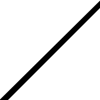
1 edge |
2 edges |

Gabor filters have received a lot of attention since they have been shown to model the spatial summation properties of the receptive fields of the so called "bar cells" in the primary visual cortex.
A Gabor function can be viewed as a sinusoidal plane modulated by a gaussian envelope. The following shows the components of a 1D function.
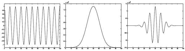 |
||
Sinusoidal |
Gaussian |
Gabor filter |
A 2D Gabor kernel can be mathematically defined as:
![]()
where
![]()
![]()
The parameters involved in the construction of a 2D Gabor filter are:
• The variance ![]() of the gaussian function
of the gaussian function
• The wavelength ![]() of the sinusoidal function
of the sinusoidal function
• The orientation ![]() of the normal to the parallel stripes of the Gabor function
of the normal to the parallel stripes of the Gabor function
• The spatial aspect ratio ![]() specifies the ellipticity of the support of the Gabor function. For
specifies the ellipticity of the support of the Gabor function. For![]() , the support is circular. For
, the support is circular. For ![]() the support is elongated in the orientation of the parallel stripes of the function.
the support is elongated in the orientation of the parallel stripes of the function.
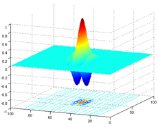
The next figure gives an example of a 100x100 pixel 2D kernel created using the above formula and ![]() = 5,
= 5, ![]() = 10,
= 10, ![]() = 0º and
= 0º and ![]() = 0.5.
= 0.5.
Using different values for wavelength, variance of gaussian and orientation, one can design a filter that is responsive to bars of a given thickness and orientation. An example of the results of the filtering process can be seen in the following example (from [1]):
 |
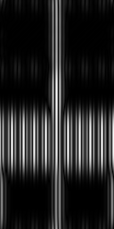 |
Input image |
Filtered image for vertical bars |
One can clearly see that the reponse of the filter at vertical bars is much higher than at vertical edges (bottom of image).
Matlab code for creating 1D and 2D Gabor filters can be found here.
[1] More details on Gabor filters, an online simulation and their applications in computer vision can be found here.