Markov Random Field Optimisation
Peter Orchard
Markov Random Fields
A Markov Random Field (MRF) is a graphical model of a joint probability
distribution. It consists of an undirected graph
 in which the nodes
  represent random
variables. Let
represent random
variables. Let  be the set of random variables
associated with the set of nodes S. Then, the edges
be the set of random variables
associated with the set of nodes S. Then, the edges
 encode conditional independence
relationships via the following rule: given disjoint subsets of nodes A, B, and
C,
encode conditional independence
relationships via the following rule: given disjoint subsets of nodes A, B, and
C,  is conditionally independent of
 given
given  if there is no
path from any node in A to any node in B that doesn't pass through a node of C.
We write
if there is no
path from any node in A to any node in B that doesn't pass through a node of C.
We write
 .
If such a path does exist, the subsets are dependent.
.
If such a path does exist, the subsets are dependent.
The neighbour set  of a node n is defined to be the
set of nodes that are connected to n via edges in the graph:
of a node n is defined to be the
set of nodes that are connected to n via edges in the graph:
Given its neighbour set, a node n is independent of all other nodes in the
graph. Therefore, we may write the following for the conditional probability of
 :
:
This is the Markov property, and is where the model gets its name. The
following diagram illustrates the concept:
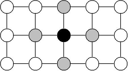
Figure 1: Given the grey nodes, the black node is conditionally
independent of all other nodes.
From this point, "node" and "variable" shall be used interchangeably.
x shall refer to a particular configuration of the set of the random variables.
A subscript will denote a particular node or subset of nodes.
The Markov property tells us that the joint distribution of X is determined
entirely by the local conditional distributions
 . But it is not clear how to actually
construct the global joint distribution from these local functions. In order to
do this, we need to look at Gibbs distributions.
. But it is not clear how to actually
construct the global joint distribution from these local functions. In order to
do this, we need to look at Gibbs distributions.
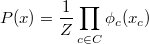
A Gibbs distribution on the graph G takes the form:
where the product is over all maximal cliques in the graph. A clique is a
subset of nodes in which every node is connected to every other node. A maximal
clique is a clique which cannot be extended by the addition of another node.
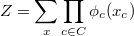
Z is called the partition function, and takes the form:
The  are usually written:
T is called the temperature, and is often taken to be 1.
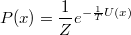
So  has the alternate form:
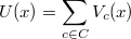
where
is called the energy. Either the  or the
 may be referred to as clique potentials.
The Hammersley-Clifford theorem states that the joint probability distribution
of any MRF can be written as a Gibbs distribution, and furthermore that for any
Gibbs distribution there exists an MRF for which it is the joint. That is to
say, Hammersley-Clifford establishes the equality of the MRF and Gibbs models.
This solves the problem of how to specify the joint distribution of an MRF in
terms of local functions: it can now be specified by defining the potential on
every maximal clique.
Optimisation
An optimisation problem is one that involves finding the extremum of a quantity
or function. Such problems often arise as a result of a source of uncertainty
that precludes the possibility of an exact solution.
Optimisation in an MRF problem involves finding the maximum of the joint
probability over the graph, usually with some of the variables given by some
observed data. Equivalently, as can be seen from the equations above, this can
be done by minimising the total energy, which in turn requires the simultaneous
minimisation of all the clique potentials.
Techniques for minimisation of the MRF potentials are plentiful. Many of them
are also applicable to optimisation problems other than MRF. For example,
gradient descent methods are well-known techniques for finding local minima,
while the closely-related method of simulated annealing attempts to find a
global minimum.
An example of a technique invented specifically for MRF optimisation is
Iterated Conditional Modes (ICM). This simple algorithm proceeds first by
choosing an initial configuration for the variables. Then, it iterates over
each node in the graph and calculates the value that minimises the energy given
the current values for all the variables in its neighbourhood. At the end of an
iteration, the new values for each variable become the current values, and the
next iteration begins. The algorithm is guaranteed to converge, and may be
terminated according to a chosen criterion of convergence. An example of this
technique in action can be seen below.
MRF Applications To Vision
Problems in computer vision usually involve noise, and so exact solutions are
most often impossible. Additionally, the latent variables of interest often
have the Markov property. For example, the pixel values in an image usually
depend most strongly on those in the immediate vicinity, and have only weak
correlations with those further away. Therefore, vision problems are well
suited to the MRF optimisation technique. Some examples of vision problems to
which MRFs have been applied are:
- Image restoration
- Image reconstruction
- Segmentation
- Edge detection
In the first 3 of these, there is a latent random variable for each pixel.
The variables range over intensity values in 1 and 2,
while in 3 the variables take on segment identifiers. In problem 4,
the variables correspond to pairs of neighbouring pixels, and their values are
binary, indicating the presence or absence of an edge. In all cases, the
neighbourhood concept of the MRF maps to the geometric neighbourhood of the
image. That is to say, the edges in the MRF graph will connect geometrically
close pixels or edges. The appropriate size of the neighbourhood depends on the
problem at hand: a larger neighbourhood has more modelling power at the expense
of greater computational demand during optimisation.
The following diagram illustrates the structure of an MRF that could be used
for image restoration. It also shows how "variables" corresponding to known
data can be incorporated into the model. The white nodes represent the unknown
true pixel values, and the grey nodes represent the noisy pixel data. Notice
that the latent variables are connected to their neighbouring pixels, but the
data points are connected only to one latent variable. This models our belief
that the estimated pixel values should depend on both the noisy data and the
estimated neighbouring pixel values.

Figure 2: Section of an MRF for an image restoration problem.
Having constructed an MRF, the clique potentials must be defined. This encodes
the relationship between variables, and so this is where we get to specify what
we want from the solution. Finding an appropriate energy function and selecting
the parameters that give an acceptable solution requires insight, as well as
trial and error. However, there are many often-used, standard energy functions
for different types of problem. For example, if the graph of figure 2 were used
for image restoration, clique potentials might take the form:


 is the observed value at data node n.
The first equation is the potential for the cliques containing one data node
and one latent node. It expresses a belief that the image is corrupted by
Gaussian noise of variance
is the observed value at data node n.
The first equation is the potential for the cliques containing one data node
and one latent node. It expresses a belief that the image is corrupted by
Gaussian noise of variance  . The second
equation is the potential for cliques containing two latent nodes. It punishes
differences between neighbouring nodes, but only up to a maximum of
. The second
equation is the potential for cliques containing two latent nodes. It punishes
differences between neighbouring nodes, but only up to a maximum of
 . This represents a statement that most regions
are smooth, but that edges are expected and so should not be punished too
harshly. The
. This represents a statement that most regions
are smooth, but that edges are expected and so should not be punished too
harshly. The  weights the importance of the
second type of potential relative to the first.
weights the importance of the
second type of potential relative to the first.
Example
Here is an example of the results from an application of MRFs to an image
restoration problem. The structure of the MRF was as in figure 2, and the
potentials were those stated above. The original image looked like this:
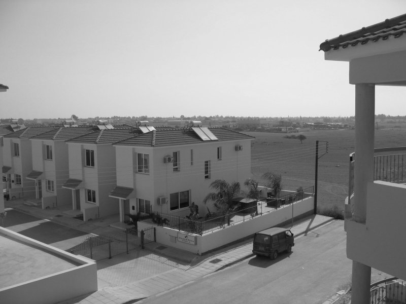
Figure 3: The original image.
Then, this matlab code was used to add Gaussian
noise to the image with covariance of 100, resulting in figure 4.

Figure 4: The image with added Gaussian noise.
Finally, this matlab code was used to smooth
the image. The parameters to restore_image were:
- max_diff = 200
- weight_diff = 0.02
- iterations = 10
The code uses a simple implementation of the ICM algorithm. It is intended as a
clear example of an MRF optimisation method, and so is not at all optimised for
efficiency. The result was figure 5.

Figure 5: The restored image.
A comparison of figures 4 and 5 shows that this restoration method has done
quite a good job of smoothing the noise from surfaces of constant or
slowly-varying intensity such as the road, the sides of buildings, and the sky.
It does not do so well with thin, sharp features; for example, the telephone
cables are almost completely removed. This is due to the energy function
punishing local differences in pixel values.
References
-
C Bishop. Pattern Recognition and Machine Learning Springer, 383-393,
2006
-
S Geman and D Geman. Stochastic Relaxation, Gibbs Distributions, and the
Bayesian Restoration of Images IEEE Transactions on Pattern Analysis and
Machine Intelligence, 6(6):721-741, 1984
-
R Kindermann and J L Snell. Markov Random Fields and Their Applications
American Mathematical Society, 1980
-
S Li. Markov Random Field Modeling in Computer Vision Springer-Verlag,
1995
-
P Perez. Markov Random Fields and Images CWI Quarterly, 11(4):413-437,
1998
-
G Winkler. Image Analysis, Random Fields and Dynamic Monte Carlo Methods
Springer-Verlag, 1995