 , where x is a variable
denoting the parameter that affects the value of
  .
Then, the rate at which
  changes when the value of x is a is
denoted:


We assume that the readers already know what derivatives are.
In vision applications, we are often interested in how a quantity changes
as some other related quantities change.
The related quantity might be the image position, or it might be
some other parameter, such as a scale factor.
The usual way to calculate or specify how the quantity changes is with the
use of derivatives.
Suppose that the quantity of interest is  , where x is a variable
denoting the parameter that affects the value of
  .
Then, the rate at which
  changes when the value of x is a is
denoted:

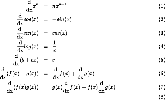
The derivatives of some commonly encountered quantities are:

where x and y are variables, b and c are numbers and  and
and  are
functions of x.
It is possible to define higher derivatives, e.g. second derivatives:

For example,

In the case of functions over an image, there are usually two (for 2D images) or three (for 3D images) variables. We then need to consider derivatives of the function with respect to all variables. This requires the use of partial derivatives.
Partial derivatives are like ordinary derivatives, except that
we keep all other variables fixed when we consider the derivative
of the function.
If there are N variables, then there are partial
derivatives with respect to all N variables.
For example, if  is a function of the image position
  ,
then we could look at the derivative with respect to either x or y.
The derivative with respect to x is denoted:

and the derivative with respect to y is denoted:

In the same way as with functions of a single variable, we can also
look at higher derivatives of  .
These second order derivatives often occur:


You might wonder where the fourth derivative function is, but it turns out that:

A useful quantity is known as the gradient.
An easy way to envision the gradient of the function  is to imagine
a X-Y grid on a flat surface and
  is the height of the surface
of interest above the flat grid surface.
The gradient is related to the slope of the surface at every point.
The direction of the gradient is the direction of the greatest uphill slope.
The size of the gradient is the amount of the slope in that direction.
Thus, the gradient function creates a vector from a scalar quantity.
The gradient is represented using the symbol
  and is
defined by:

The gradient has a value everywhere (on smooth surfaces) as you would expect: a smooth surface has a slope everywhere. The direction of the gradient is defined using the unit vector calculation:

and the magnitude of the gradient is just the length of the gradient vector:

A common second order derivative of a image quantity  is called
the Laplacian, which is defined as:

This is the sum of two second order partial derivatives, and is a scalar rather than a vector quantity.
Finally, we defined the derivative quantities as if the functions that they apply to are continuous, whereas often we are working on a quantized image grid. Therefore, the mathematical definition of the derivative:

has a problem -- we cannot really take the limit  ,
as we have only a quantized set of values to work with:
  .
The smallest possible value is h=1 as a division by zero occurs at
the next smallest possible value h=0.
Therefore, the derivatives are often approximated by

or

One could use larger neighborhoods around the point to get a better estimate of the derivative at x, which would have to trade off accuracy against the fact that larger neighborhoods are also more likely to include unrelated surface details. The estimation of derivatives is not always ideal, so a variety of numerical techniques have been developed, but they are not discussed here.


