

Next: Alternate derivation: from the
Up: Essential and fundamental matrices
Previous: Essential and fundamental matrices
To describe the relationship between R,
 ,
A1, and A2 more
exactly, and to connect the above equations with those found in
[6], we offer the following algebraic derivation.
Recall that a point
 produces an image
 through the equation
 .
Without loss of generality, we can assume that
 is given
with respect to the first camera's coordinate frame to yield the following
two imaging equations:
where  and
and  are scale factors,
 is the
 identity matrix and
 is the
 null
vector. By letting
![$\ensuremath{{\bf M}} = \left[\matrix{\ensuremath{{\bf\hat M}} ^T & 1}\right]^T$](img170.gif) (
(
 is
is
 ), we
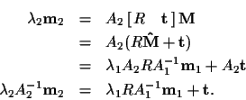
achieve the following relation:

(8) (9)
Geometrically, this equation says that the vector on the left is a linear
combination of the two vectors on the right. Therefore, they are all
coplanar, and the vector
 is perpendicular to that plane:
which is identical to (6).
Similarly, the vector
 is perpendicular to the vectors in (8):
This is a surprising result because it gives us a new and equivalent
expression for F:
![\begin{displaymath}F =[A_2 \ensuremath{{\bf t}} ]_x A_2 R A_1^{-1},
\end{displaymath}](img177.gif) |
(10) |
which shows that F can be written as the product of an
anti-symmetric matrix
![$[A_2 \ensuremath{{\bf t}} ]_x$](img178.gif) and an invertible matrix
A2 R A1-1 [4].
and an invertible matrix
A2 R A1-1 [4].


Next: Alternate derivation: from the
Up: Essential and fundamental matrices
Previous: Essential and fundamental matrices
Stanley Birchfield
1998-04-23
![]() ,
A1, and A2 more
exactly, and to connect the above equations with those found in
[6], we offer the following algebraic derivation.
,
A1, and A2 more
exactly, and to connect the above equations with those found in
[6], we offer the following algebraic derivation.
![]() produces an image
produces an image
![]() through the equation
through the equation
![]() .
Without loss of generality, we can assume that
.
Without loss of generality, we can assume that
![]() is given
with respect to the first camera's coordinate frame to yield the following
two imaging equations:
is given
with respect to the first camera's coordinate frame to yield the following
two imaging equations:
![\begin{eqnarray*}\lambda_1 \ensuremath{{\bf m}} _1 & = & A_1 \left[\matrix{\ensu...
...matrix{R & \ensuremath{{\bf t}} } \right] \ensuremath{{\bf M}} ,
\end{eqnarray*}](img165.gif)

![]() is perpendicular to the vectors in (8):
is perpendicular to the vectors in (8):
