Bernstein-basis curves and sculptured surfaces
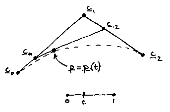
Below is the curve from Problem Sheet 2. This construction is called the de Casteljau construction, and this particular example with three control points gives a parabola. (I have changed the control point labels from p in the problem sheet to c for control.)

This construction generalizes to any control track. We join the points that are a fraction t along each leg to the corresponding points on the next legs. This gives a track with one fewer points on then the one we started with. We then do the same to that track and so on until we get down to a single point - the point on the curve at parameter value t:
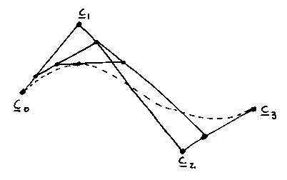
The result is a Bézier (or less commonly de Casteljau) curve (they both invented it).
If you do the maths, the equation of the curve turns out to be:

where

which is to say the i-th term of the n+1 terms in the binomial expansion of

which, of course, is a very fancy way of writing the number 1...
(Note that we define 0! = 1.)
So. What we are doing is to multiply each control point by a weight (the B things that all add up to 1) and add up the results to make the point on the curve, p(t). As t goes from 0 to 1, the point p sweeps along the curve.
The weights B are not called B because they are from the binomial expansion, but after Bernstein, who invented them for this sort of thing. They are known as the Bernstein basis functions and the whole of the mathematics of Bézier curves and surfaces (and others below) is founded on them.
The picture above has four control points,
 . Below are the four Bernstein
weights that would be used to multiply them.
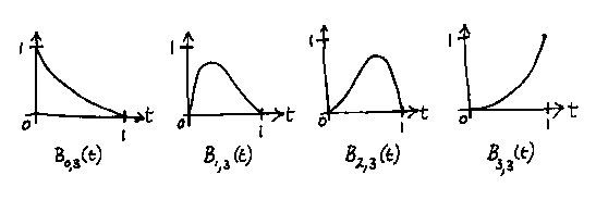
Note that these are symmetrical. If we go back, for a moment, to an ordinary (non-Bernstein) parametric polynomial like

then we can treat the powers of t as `weights' being applied to some points in space (the a values; the coefficients of the powers of t). If we plot how the powers of t behave they go like this:
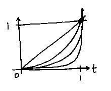
Which (apart from the constant term) have no obvious symmetry about them, and tell us little about what effect each a vector will have on the shape of the curve. But the Bernstein weights...
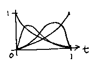
...do give us some intuition as to what might happen. For example, at the start the weight for the control point labeled 0 is 1 and for all the others is 0. We would thus expect the curve to start at that point and to move away from it [in fact, doing the algebra proves that the curve is tangential to the control track at the start (and end)]. The weight on the point labeled 0 then diminishes, while the weights for the other points rise, so we would expect the curve to tend to go towards those points. Finally, the weighting functions are symmetrical, so we would expect the curve to end at point n in the same way as it started at the point labeled 0.

The curve is tangential to the control track at the ends, and tends towards the other control points in the middle; the middle control points act like handles on the curve - as we move them the curve follows along, but always stays smooth.
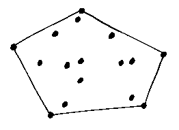
Also, as was demonstrated by the answer to Question 4 on Problem Sheet 2, the curve cannot move outside the convex hull of the control points. The convex hull of a set of points is the convex polygon you'd get if you let an elastic band snap tight around them:
Joining Bernstein-basis Curves
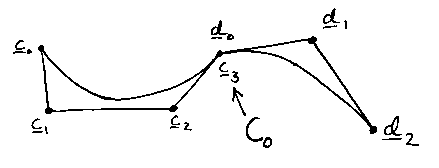
We can obviously get  continuity
just by joining two control tracks end-to-end:
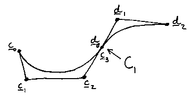
And  continuity by ensuring
that the end of one control track is colinear with the start of the
next (because the tracks are tangent to the curves at their ends):
We can join the track onto itself to make a closed curve with an angled join...
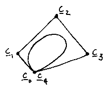
...or a smooth one:
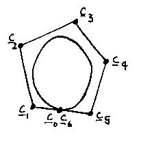
Suppose we want to make a long complicated curve with lots of control points:
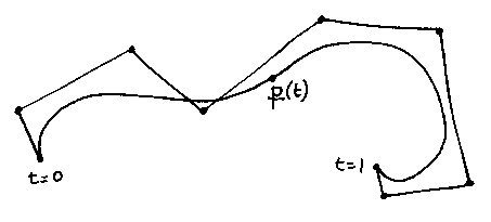
This will certainly work, but it will generate a very high-degree polynomial (that is there will be high powers of t in the Bernstein-basis functions). The Bernstein basis has the nice property that it is very numerically stable, so rounding errors in the computer with the high-degree terms will not be a problem, but the curve may take a while to compute.
There is another problem. If we are designing a complicated shape, then we will probably get one bit right (by moving the control points, say), then go on to the next bit. But when we move any control point, we change the shape of the whole curve, so we may destroy previous painstaking work. This is because the whole curve is a single polynomial function.
The fact that the whole high-degree curve is a single
polynomial function also means that it has a very high degree of
continuity - we can differentiate it lots of times without the
derivatives becoming discontinuous. Generally, continuity is a good
thing, but few applications need more than
 continuity.
We can take advantage of this to generate a spline instead of a single Bézier polynomial curve - that is a collection of Bézier curves joined smoothly all using just one control track.
We start by chosing values of t at which one curve will end and the next start:
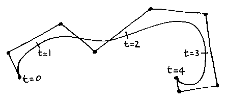
It is convenient to abandon the convention that t goes from 0 to 1, simply so that these intermediate values can be whole numbers.
The equation of the spline of Bézier curves (which is called a B-spline, not - as you might think - as an abbreviation of Bézier-spline or even Bernstein-spline, but of beta-spline...) looks by now familiar:

but the weights, now called N, are different:

Which looks, and is, pretty horrendous. Note in particular that the definition of N is recursive - it is defined in terms of simpler versions of itself.
The value of k is the degree that the joined-up Bézier curves will have.
The values of r are the values of t at which one Bézier curve will end and the next start (0, 1, 2, 3, 4 in the picture above - these individual values of t are called knots and the list of values is called the knot vector).
How do we terminate the recursion? That is to say, what happens when k = 1?

Which is a square-wave with the value 1 when t is between two knots, and 0 when it is outside them. The result of then doing the recursion is effectively to integrate and to smooth those square waves until we end up with weights that look like this:

After all that, it's fairly easy to loose sight of the fact that what we're doing is to apply these weights to the control points and to add up the results. Note that the weights have values of 0 for parts of the range of t along the spline. That means that the corresponding points can have no influence over the spline for those t values. This is what we wanted to achieve - the spline is now local, and we can (if we set it up right) move control points at one end without affecting the other.
How do we set it up right? Well, unfortunately we have to do some fixes to make the weighting functions fill up the ends. Generally, we have n + k + 1 knots, and we duplicate knots at the ends of the knot vector to achieve this:

So we get knot vectors like (0,0,0,1,2,3,4,4,4).
The final fix we need is a definition:

Which stops things going haywire when the parameter value passes through the knots.
The best thing to do with all the above, once you've got the hang of it, is to code it into your program, test it to make sure it's OK, then let the computer worry about it from then on...
Despite the extreme nastyness of the mathematics of B-splines, it
reduces to the more elegant Bézier form when you choose
a value of k that bunches all the knots at the ends,
for example
(0,0,0,0,1,1,1,1). So B-splines are a both a genralization of
Bézier/Bernstein curves and a collection of them joined with a
required continuity.
Bernstein-basis sculptured surfaces
The idea of a control track generalizes to a control grid (in red) and we can build a Bernstein-basis sculptured surface or patch:
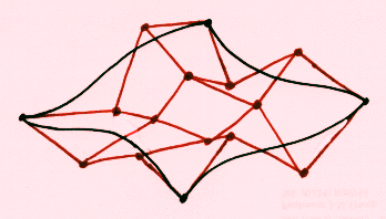
If this is a Bézier patch it has the formula:

And if it is a B-spline patch (which once again is just a collection of it Bézier patches joining with a required continuity) it is:

A small curiosity is that the de Casteljau geometrical construction continues to work through all of these extensions and generalizations. If, instead of the ladder-sliding-down-a-wall idea that we had in the two-dimensional case, we allow a quadrilateral to slide about with its corners in the surfaces of 4 other quadrilaterals:
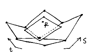
The positions of the corners, and the position of our point in the
surface, p, are governed by s and t in
an exactly analogous manner to the two-dimensional case, and the
recursive nature of the construction still applies.
Strengths and weaknesses of Bernstein-basis curves and sculptured surfaces
 You can't design a parametric
polynomial patch by specifying the coefficients. If you try to fit a
surface through too many points it goes all wiggly and unstable.
So the control grid gives you a nice set of handles for building
surfaces.
 Bernstein-basis curves and surfaces
are invariant under affine transforms. An affine transform is
a rigid-body motion (that is a translation or rotation), a
change of scale, or a linear shear. So. If you apply the
transformation to the control grid and recompute the surface, you get
the same thing as if you'd transformed the original surface.
This is very convenient, as it means that you can design the surface
in one place and copy it elsewhere just by copying the control grid.
 Bernstein-basis curves and surfaces
stay within the convex hull of their control grid. This is useful, as
the convex hull is quite easy to compute, and, when we've got it, we
know where the curve or surface isn't. Thus we can tell that it
won't collide with other parts of the design, for example.
 Bernstein-basis curves and surfaces
are very numerically stable (far more so than polynomials written out
in the usual way).
 Degree elevation. It is
algebraically quite simple to take a Bernstein-basis polynomial
and to increase its degree without altering its shape. Why bother?
Well, the control grid moves if you do this, and the number of points in
it increases. It moves nearer to the curve, becoming a better
approximation to it. It is very useful to have a simple way of making a
variety of approximations to a shape of increasing accuracy.
 Bernstein-basis curves and surfaces
are very widely used. This is the same as one of the advantage of b-rep
geometric modellers.
 Bernstein-basis curves and surfaces
are expensive to calculate. They take a time that is
 to compute.
 Bernstein-basis curves and surfaces
can be hard to understand...
 The control grid looks easy
to work with, and it certainly is easier than working out the
coefficients of a conventional polynomial, but it isn't that easy and
intuitive to design with.
 It is very difficult to compute the
curve of intersection between two Bernstein-basis surfaces:
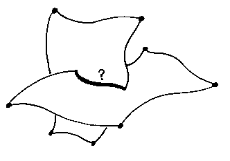
 For practical engineering design,
we often need triangular patches; these are hard to formulate.
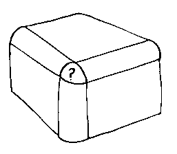
 It's not very easy to put in
fillets and radii in a design, though lots of work has been done on
this.
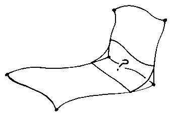
 Though we can make car bodies and
aeroplane wings from Bernstein-basis surfaces, we can't make simple
shapes like spheres and cylinders! To do so exactly would need
Bernstein-basis surfaces of infinite degree. This brings us finally
to...
NURBS
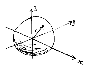
The implicit equation of a sphere centred at the origin is:

which is nice and simple. The simplest parametric equation of a sphere uses sines and cosines (think of latitude and longitude). But our Bernstein-basis patches can't do a sphere at all.
What is the reason for this? If you consider a general parametric equation of a surface (which we expand out to formulae for x, y and z for once, rather than leaving them in vector form):

you will see that we have three equations with five unknowns (x, y, z, s and t). We can (in principle; in practice the algebra is very hard) eliminate s and t giving us one equation in x, y and z. So, we can always convert from a parametric polynomial to an implicit polynomial.
BUT THERE IS NO GUARANTEE THAT YOU CAN GO THE OTHER WAY. You can't always convert from an implicit polynomial to a parametric one. There are `more' implicit polynomials than parametric ones (in fact, there are an infinite number of both, of course, but there isn't a one-to-one mapping between the two sets). Even some very simple implicit polynomials like the sphere and cylinder have no direct parametric equivalents.
NURBS are Bernstein-basis curves and surfaces that get us out of this tight spot. NURBS is an acronym for Non-Uniform Rational B-Spline. What you do is to take the B-Spline patch formula:

and divide the weights by another set with a different knot vector:

To get spheres and cylinders and so on the knots have to have unequal gaps [so instead of (0,0,0,1,2,3,4,4,4) you get things like (0, 0, 0, 1.2, 2.765, 3.7, 4, 4, 4)] - hence the non-uniform bit; we have one knot vector for the top of the division, and another for the bottom. It's called rational because it now involves a division, and it's still a B-spline with all the properties listed above.
It's still the case that we can't turn every implicit polynomial into a NURBS, but at least we can now do the simple shapes like cylinders and cones which are vital for engineering.
Integrating surface patches and b-rep modellers
Putting surface patches into a b-rep modeller is (in principle at least) fairly simple: topologically they are rectangular, so the the Euler-Poincaré formula sees them as rectangles. The problem is rather similar to that of getting cylinders into the modeller by pretending that they are prisms with curved ends.
We can use the convex hull property to check if surfaces might collide - this is fast if most don't, and, in a well-designed model, they won't often. Problems start when we have to work out the actual intersection curves between patches and other curved surfaces or other patches, as the algebra gets hard (though not impossible). However approximations are often used simply because they're faster.
The temptation to use NURBS for everything (including flat planes), because that means that you have only one surface type to deal with is strong. But this can be very inefficient.
Diversion: Warnock's rendering algorithm, and ray-tracing.
© Adrian Bowyer 1996