Set-theoretic or Constructive-solid-geometry Modellers
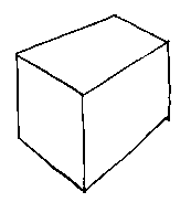
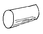
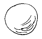
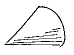
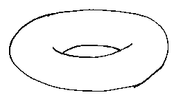
Consider the simple primitives that we used for b-rep modelling: the plane, the cylinder, the sphere, the cone, and the torus:


If we could treat these as a sort of three-dimensional Venn diagram we could make many engineering shapes by unioning, subtracting, and intersecting them together. Doing this is set-theoretic solid modelling. It is such an intuitive way for people to build shapes that it is often used as an input method for b-rep modellers, but here we will be concerned with how to deal with the set-theoretic description of shapes directly, without translating them to b-rep.
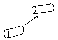
Firstly, we need some way of getting the primitives in the right place. We use translation:
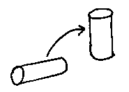
Rotation:
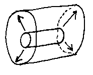
And scale change:
We then put the model together bit by bit by building a set-theoretic expression. Say this is the shape we want:
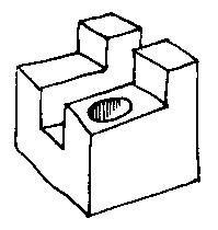
Then we put the pieces together in pairs, which the computer builds into a tree:
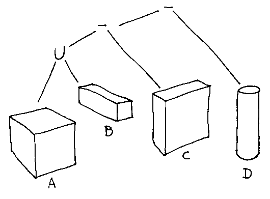
The - operator is useful because people find it easy to think with, but often internally it is converted so that the computer's version of the model has only unions and intersections:
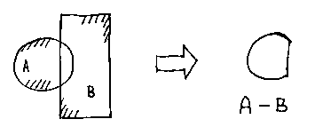
A - B is the same as...
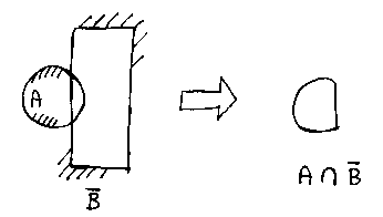
...the intersection of a with the complement of B.
Set-theoretic modellers are sometimes called Constructive Solid Geometry modellers (CSG for short), or Boolean modellers.
Why Boolean? Consider the binary numbers 0101 and 0011. The Boolean AND of these is 0001, and the OR of them is 0111. AND behaves just like intersection, and OR behaves just like union.
This allows us to program a membership test: a test to see if a given point is in the solid part of a geometric model or in the `air' part. Here is a point in the union of two sets:


Here are the other possibilities:


We can extend this to find out if the point is inside or outside a set-theoretic geometric model of any complexity.
But how do we know the INs/OUTs (or TRUEs and FALSEs) for the point and the individual primitives?
Here's how we handle a line in two dimensions (a three dimensions plane is just the same; it merely requires an extra term in z):
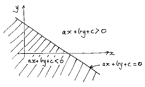
We treat the line as an inequality, giving us a half-plane (just like the ones in Problem Sheet 3).
In two dimensions we can intersect 4 of these to make a rectangle (or any convex quadrilateral):
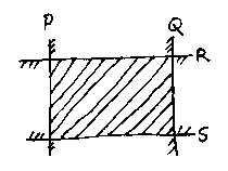
In three dimensions, of course, 6 will make a cuboid.
But the really powerful thing is that we can use any function of x and y (and z in three dimensions) to make shapes, just by treating it as an inequality:
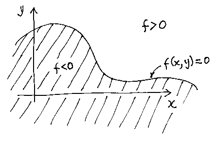
It is easy to write down the inequalities for spheres and cylinders and the like, but what about more general shapes (such as the ones we needed NURBS for in b-rep modelling)? And what about translating and rotating such shapes to get them in the right place?
Recall that to find the distance from a point to a straight line all we need to do is to put the point's coordinates into the expression for the line:
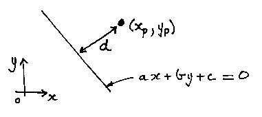

As long as the line is normalized:

We can use this fact to build more complicated shapes. For example a disc:
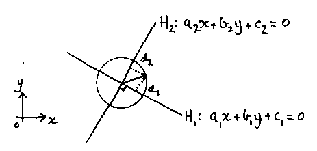
Can be made from any two lines that cut at right angles at its centre. Pythagoras tells us that the disc's inequality must be:

where R is the radius we want.
In three dimensions the lines become planes, and the shape becomes an infinitely long cylinder centred on the two planes' line of intersection.
We can use distances to planes to build up complicated three dimensions shapes in this way. The great advantages of this are that: 1) it isn't too hard to think about when you get the hang of it, and 2) the shapes can be translated and rotated merely by translating and rotating the planes.
Ray-tracing set-theoretic models
Again, in two dimensions for simplicity, consider this hamburger shape:
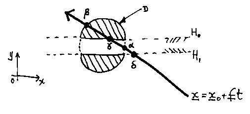
It is made from two half-planes and a disc:

Though the computer will remove the difference operator:

Suppose we want to find the point where a ray first hits the model. The ray is a parametric straight line.
The steps are these:
1. Compute the parameter (t) values at the intersections between the ray and the individual primitives:

2. Sort by increasing parameter value t:

3. Membership test the (x,y) values corresponding to each value of t in order till a TRUE is hit. For example

No, so this is a FALSE.

No, so this is a FALSE.

This must be TRUE as this was the surface that generated the intersection; for each such case we put in TRUE immediately without any calculation.
So our membership-test expression is:

And the point is indeed not the place where the ray strikes.
If we continue we will eventually find that the point
corresponding to the t value of
 will give us a TRUE.
All this works just as well in three dimensions, so we can ray-trace into a set-theoretic solid model and make pictures. Rays are often useful for other things too, like working out how far something can move before it hits the model.
But there's a problem. The picture may have half a million pixels; the model may have thousands of primitives (the oil refinery has about 1200); we may want many rays per pixel for shadows, reflections, and so on. Each ray has to be intersected with all primitives. Each membership test takes a time proportional to the square of the number of primitives. So the time taken will be half a million times the cube of the number of primitives - perhaps a billion - times some constant, which better be damn small...
In fact, if this were all we could do, we'd have to wait years for a picture.
How can we improve things? Consider a model (again in two dimensions for clarity) that is two quadrilaterals (the shaded area):
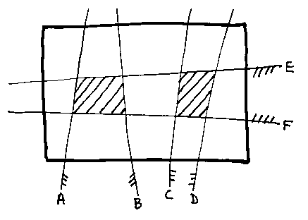
The model is: 
What we do is to put a box round the model (the heavy rectangle), then recursively divide it. The next picture might be the first chop. Consider what happens in the left half.
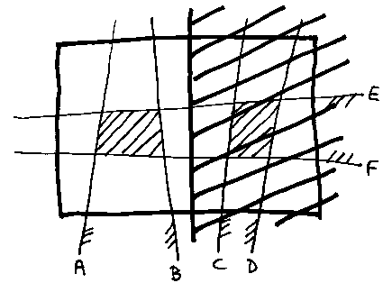
On the left we've thrown away C and D. C contributed all `air' to the left half; D contributed all solid. So on the left only the model is:

Now, anything intersected with air must be air, no matter how complicated it is. So this simplifies to:

Anything unioned with air is just itself, so we finally have...

... as what is in the left hand side. This simplification is called pruning. It really comes into its own when we repeat the division recursively. We end up with a tree of boxes that each contain a much-simplified version of the original set-theoretic expression. In many cases they will just contain the null set (air) or the universal set (solid) - as simple as one could get. The next picture shows such a tree of boxes with the simplified contents of two of them labeled.
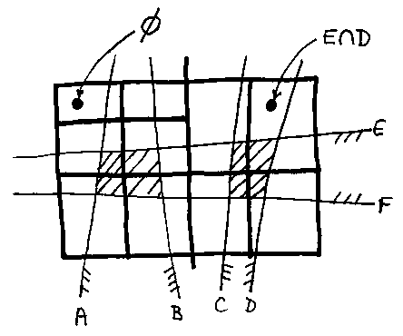
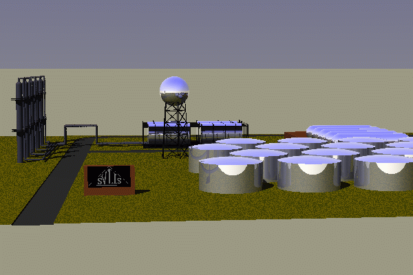
This can all be done just as easily in three dimensions. We get a solid cuboid volume that is recursively divided into many smaller cuboids. This both localizes and simplifies the model. (`Localizes' means that the boxes tell you where in space the bits of the model are.) This structure is generally very useful for many things, but in particular it makes ray-tracing tractable. The rays run through the simple boxes, and only a few (or often no) calculations need be done in each box. The refinery picture (which was generated from a set-theoretic model in exactly this way) took about 3 minutes to ray-trace on a PC:
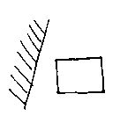
But we have glossed over a problem. To do this, it is necessary to be able to tell if a box is in air for a half-space:
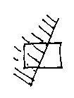
Or is part-air and part-solid:
Or is all solid:
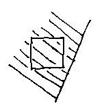
This is pretty easy for a planar half space (like those three figures of lines in two-dimensions). But wahat about curved surfaces? Well, a sphere, or disc in two-dimensions...
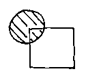
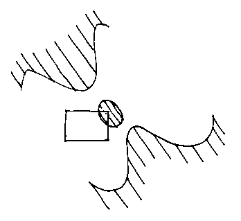
...is quite easy too. But in general a single implicit polynomial inequality can fall into several lumps and be very hard to categorize boxes against:
Interval arithmetic
One way to approach the problem - and a powerful general technique for getting ball-park answers to lots of problems - is to use interval arithmetic. An interval is a single section of the real line. For example, we might have an inteval [0.5, 1.5], which means all the numbers between 0.5 and 1.5. We can do arithmetic with these things. So, that interval [0.5, 1.5] can be added to the interval [2, 3] to give the result [2.5, 4.5]:

What this is saying is that if we add any number in [0.5, 1.5] to any number in [2, 3] we must get an answer somewhere in [2.5, 4.5].
Extra work: Can you work out the rule for adding two intervals [a, b] + [c, d]? (Remember that the ends may be negative.) How about subtraction? Multiplication? Raising to a power (even powers are not the same as odd)? Most difficult of all, what about division?
How might interval arithmetic help with the box classifications against implicit inequalities? As an example consider a function of a single variable, x:
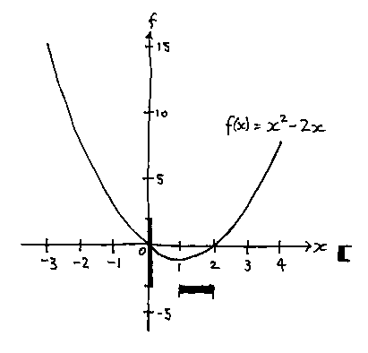
What values might the function take for all possible values of x in [1, 2]? Well. If

Then

and

so

Which is telling us that, for that range of x values, the function generates values that lie somewhere in [-3, 2]. Note that, by looking at the function, we can see that the actual range of values that it takes is [-1, 0], which is indeed in [-3, 2]. But the technique hasn't given us an exact answer; it has given a conservative answer that is guaranteed to contain the exact answer.
But our original problem was to classify a box against an implicit inequality. Let's look at a two-dimensional example:
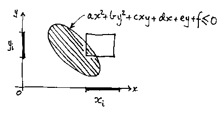
A box is just two intervals. Suppose we have the quadratic solid (an ellipse, maybe):

Then to find if a box is all true (that is all solid) for the inequality, or all false (i.e. all air), or bits of both (i.e. some of the surface of the inequality is in the box and it's both solid and air), we just put the intervals into the expression and evaluate it to give an interval, i, as the result:

If i is wholly negative, we know that the box must be all solid. If i is wholly positive, we know that the box must be all air. If i contains 0, then there may be some of the surface of the inequality in the box. Note that in this case we're not sure, because of the conservative nature of interval arithmetic.
But this lack of certainty doesn't matter for our divide-and-prune algorithm. It can categorize most implicit inequality primitives against boxes, and the ones that it's not sure about remain in the set-theoretic expression. But as the boxes get smaller and smaller, the interval arithmetic gets less and less conservative (in the limit, when the intervals have no length, the box becomes a point and the answer is exact for that). So we just keep dividing and pruning.
We can also use the scheme for our implicit primitives made up by doing arithmetic on plane expressions. Here's the ellipse again, but formed like that:
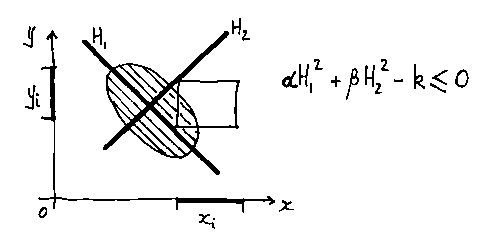
If

Then we can put the box intervals into those expressions:

Giving two intervals, then put those into the expression for the ellipse:

In general using planes in this way gives tighter bounds on the answer than doing the interval arithmetic for the multiplied-out expression.
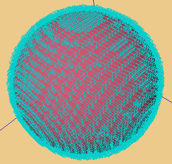
Here's an example from a real (though simple) geometric model. It's an oblate spheroid (Oh. All right. A Smartie) - a single implicit polynomial inequality. The modeller was instructed to find small boxes containing surface using interval arithmetic as described. The dark-blue lines are the coordinate axes.
Blends for implicit-inequality solids
As has been mentioned before, it is a common requirement of a geometric modeller that it should smooth off some sharp edges and corners in models by creating blends and fillets. Many different (and not necessarily compatible) solutions to this problem have been proposed for both b-rep and set-theoretic modellers.
Here is one method that works well for implicit-inequality-based set-theoretic modellers. It was devised in the Second World War by R.A. Liming as a way of designing aircraft fuselages by hand years before people thought of CAD and CAM. If you have expressions for four arbitrary straight lines:
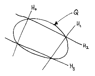
And you form the quadratic:

It will always pass through the four intersection points shown (note
there are two more intersection points that are not relevant). To prove
this to yourself remember that the quadratic curve is Q = 0.
Think which H expressions need to be 0 to make Q 0.
Different values of  between
0 and 1 give different
curves, but they all pass through the four points.
If we collapse two of the lines together:
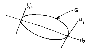
And rewrite the expression for the quadratic:

We get a family of quadratics which are tangential to the first two lines where the third cuts them.
We can use this to put a fillet in a corner:
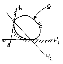
If we get the signs right (so that Q is a bubble when treated as an inequality, rather than solid in the middle) we can make the sharp-cornered object

into the smoothly-filleted object

As long as the line which decides where the tangencies will
be,  , is (when treated as an
inequality) solid to the left.
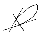
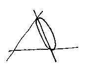
We can use  to control the
blend. This is what we get for values near to 0:
And this for values near to 1:
But the beauty of this scheme is that it works in three-dimensions too, and with any implicit functions. So we can blend curved surfaces as well as flat ones:
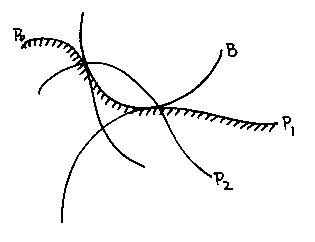
We can even put blends on blends. The only problem is that the degree of the blend polynomial increaces as we make more complicated ones.
Here is such a blend forming a smooth fillet between pipes joining at an angle:
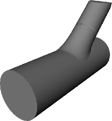
So far, we have been filleting corners:
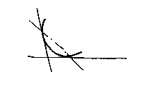
But ther is another sort of blend needed, a gap blend like the junction between the neck and the body of a wine bottle:
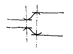
The formulation for achieving this was invented by Dayong Zhang, who was a student at Bath:
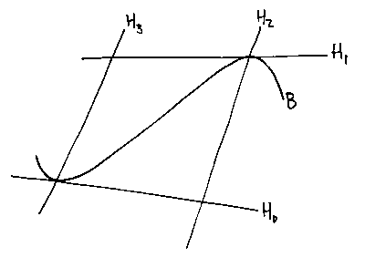
The blend is:

If the original surfaces to be blended are linear, then this gives a cubic (as would be expected, as the blend contains an inflexion). But once again the method works for any implicit functions.
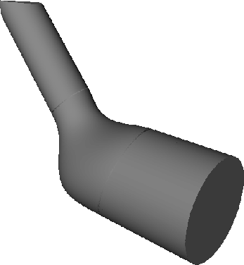
Here is a gap blend between two cylinders of different diameters and with offset axes. These gap blends fill lots of the requirements that were solved using duct-type modelling.
© Adrian Bowyer 1996