


Next: Minimisation
Up: Variational Optic Flow
Previous: Variational Optic Flow
The Variational Model
Before deriving a variational formulation for our optical flow method,
we give an intuitive idea of which constraints in our view should be
included in such a model.
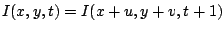
- Grey value constancy assumption.
Since the beginning of optical flow estimation, it has been assumed
that the grey value of a pixel is not changed by the displacement.
 |
(1) |
Here
 denotes a rectangular image
sequence, and
denotes a rectangular image
sequence, and
 is the searched displacement vector
between an image at time
is the searched displacement vector
between an image at time  and another image at time
  .
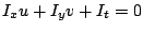
The linearised version of the grey value constancy assumption yields
the famous optical flow constraint [11]
.
The linearised version of the grey value constancy assumption yields
the famous optical flow constraint [11]
 |
(2) |
where subscripts denote partial derivatives. However, this linearisation
is only valid under the assumption that the image changes linearly
along the displacement, which is in general not the case, especially
for large displacements. Therefore, our model will use the original,
non-linearised grey value constancy assumption (1).
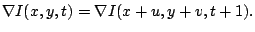
- Gradient constancy assumption.
The grey value constancy assumption has one decisive drawback:
It is quite susceptible to slight changes in brightness,
which often appear in natural scenes. Therefore, it is useful to
allow some small variations in the grey value and help to determine
the displacement vector by a criterion that is invariant under
grey value changes. Such a criterion is the gradient of the
image grey value, which can also be assumed not to vary due to the
displacement [18]. This gives
 |
(3) |
Here
 denotes the spatial
gradient. Again it can be useful to refrain from a linearisation.
The constraint (3) is particularly helpful for translatory motion,
while constraint (2) can be better suited for more complicated
motion patterns.
denotes the spatial
gradient. Again it can be useful to refrain from a linearisation.
The constraint (3) is particularly helpful for translatory motion,
while constraint (2) can be better suited for more complicated
motion patterns.
- Smoothness assumption.
So far, the model estimates the displacement of a pixel only
locally without taking any interaction between neighbouring pixels
into account. Therefore, it runs into problems as soon as
the gradient vanishes somewhere, or if only the flow in normal
direction to the gradient can be estimated (aperture problem).
Furthermore, one would expect some outliers in the estimates.
Hence, it is useful to introduce as a further assumption the
smoothness of the flow field. This smoothness constraint can
either be applied solely to the spatial domain, if there are
only two frames available, or to the spatio-temporal domain, if
the displacements in a sequence of images are wanted. As the
optimal displacement field will have discontinuities at the
boundaries of objects in the scene, it is sensible to generalise
the smoothness assumption by demanding a piecewise smooth
flow field.
- Multiscale approach.
In the case of displacements that are larger than one pixel per
frame, the cost functional in a variational formulation must be
expected to be multi-modal, i.e. a minimisation algorithm could
easily be trapped in a local minimum. In order to find the global
minimum, it can be useful to apply multiscale ideas: One starts
with solving a coarse, smoothed version of the problem by working on
the smoothed image sequence. The new problem may have a unique minimum,
hopefully close to the global minimum of the original problem. The
coarse solution is used as initialisation for solving a refined
version of the problem until step by step the original problem is
solved. Instead of smoothing the image sequence, it is more efficient
to downsample the images respecting the sampling theorem, so the model
ends up in a multiresolution strategy.
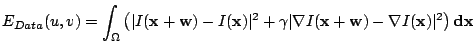
With this description, it is straightforward to derive an energy
functional that penalises deviations from these model assumptions.
Let
 and
. Then the global
deviations from the grey value constancy assumption and the gradient
constancy assumption are measured by the energy
and
. Then the global
deviations from the grey value constancy assumption and the gradient
constancy assumption are measured by the energy
 |
(4) |
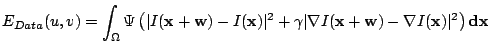
with  being a weight between both assumptions. Since
with quadratic penalisers, outliers get too much influence on the
estimation, an increasing concave function
being a weight between both assumptions. Since
with quadratic penalisers, outliers get too much influence on the
estimation, an increasing concave function  is
applied, leading to a robust energy [6,12]:
is
applied, leading to a robust energy [6,12]:
 |
(5) |
The function  can also be applied separately to each of these
two terms. We use the function
can also be applied separately to each of these
two terms. We use the function
 which
results in (modified)
which
results in (modified)  minimisation. Due to the small positive
constant
minimisation. Due to the small positive
constant  ,
,  is still convex which offers advantages
in the minimisation process. Moreover, this choice of does not
introduce any additional parameters, since is only for
numerical reasons and can be set to a fixed value, which we choose
to be
is still convex which offers advantages
in the minimisation process. Moreover, this choice of does not
introduce any additional parameters, since is only for
numerical reasons and can be set to a fixed value, which we choose
to be  .
.
Finally, a smoothness term has to describe the model assumption
of a piecewise smooth flow field. This is achieved by
penalising the total variation of the flow field [15,8],
which can be expressed as
 |
(6) |
with the same function for as above. The spatio-temporal gradient
 indicates that a
spatio-temporal smoothness assumption is involved. For applications with
only two images available it is replaced by the spatial
gradient.
indicates that a
spatio-temporal smoothness assumption is involved. For applications with
only two images available it is replaced by the spatial
gradient.
The total energy is the weighted sum between the data term and
the smoothness term
 |
(7) |
with some regularisation parameter
 .
Now the goal is to find the functions
.
Now the goal is to find the functions  and
and  that minimise
this energy.
that minimise
this energy.
Next: Minimisation
Up: Variational Optic Flow
Previous: Variational Optic Flow
Thomas Brox
2004-06-29