Introduction
Traditionally there have been two vision based methods for recovering 3-D data; stereo vision and structure from motion. (For an excellent background into geometric vision and in particular stereo vision, see the 'Multi-Sensor Geometries' section of the CVonline compendium of computer vision.) However, in current computer vision research, combining both spatial and temporal image information is becoming increasingly popular as a way of improving the robustness and computational efficiency of recovering the 3-D structure of a scene.
Temporal Stereo: A Structure from Motion Perspective
Structure from motion solutions to 3-D data recovery are inherently temporal, usually using a monocular sequence of images. Recent research, such as the Vanguard project, has demonstrated robust methods of using such techniques, even when the camera motion has to be recovered simultaneously with the 3-D data structure. However, a couple of failings that these algorithms suffer from are:
Researchers have tackled the issue of augmenting structure from motion vision systems with stereo information. This can help overcome problems such as resolving the `results up to a scale' problem and the extra information from stereo correspondences can increase the robustness and accuracy of the 3-D data recovered from the scene. Some algorithms of this type are; [4, 5, 6, 7] which are feature based, and [8, 9, 10, 11] which produce dense depth data using optical flow from spatial and temporal image gradients.
For example in [8], the algorithm establishes dense disparity maps for the left and right image sequences independently using temporal and spatial image derivatives. However, the depth from motion disparity maps are only correct up to a scale. The correct `disparity scale' is established by performing a search over a range of scales, seeing which scale maximises a correlation measure between the two left and right disparity images.
In the case of the `feature tracking' types of algorithms, Kalman filtering is very often employed as a robust means of estimating and predicting the 2-D and 3-D motions of the features. These types of algorithms usually employ conventional stereo algorithms along side the motion tracking. For example; the algorithm in [4], given a stereo camera system and a set of possible stereo matches, the algorithm generates a set of virtual objects, one for each possible match. This recursive algorithm then uses Kalman filtering to predict the motion of the virtual objects through the sequence. Incorrect stereo matches are identified because their tracks in 3-D space do not follow their Kalman filter predicted paths and as such can be rejected. As sequences of stereo images progress, the variances used in the Kalman filter get smaller as more stereo correspondences are resolved and this in turn aids matching new/unmatched tokens.
Temporal Stereo: A Conventional Stereo Perspective
Tackling the temporal stereo problem from a different perspective, leads us to a set of vision algorithms which exploit various aspects of temporal image data to improve the robustness of conventional depth from stereo algorithms.
Conventional stereo algorithms reconstruct the structure of a scene from two images taken from slightly differing viewpoints. Providing the stereo algorithm can identify corresponding points/regions in the left and right images, then the location of those points in the images, combined with camera calibration information, allows accurate 3-D data for the real world to be recovered.
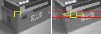
Assuming that calibration information for the stereo cameras is available to our algorithm, we are free to exploit the epipolar constraint to reduce the matching process for finding corresponding points from 2-D searching (whole images) to 1-D searching along corresponding epipolar lines. Area based stereo algorithms identify possible matches for a point of interest in one stereo image using a similarity metric (e.g. correlation) to find corresponding regions on an epipolar line in the other stereo image:

Figure 1, Searching along an epipolar line for corresponding image regions.
[12, 13, 14, 15] can all be classed as sudo-temporal stereo vision algorithms. They have been developed with robust solutions to the stereo correspondence problem in mind, taking monocular sequences of images as their input. The input sequences are usually produced by a single camera undergoing a carefully controlled translating or rotating motion to capture various views of a scene from known positions. Stereo image pairs are produced by selecting and pairing different images from the monocular input sequence.
Because solving the correspondence problem for a stereo image pair with a wide baseline is difficult, these algorithms initially start with a stereo pair of a short baseline which can be matched easily because of the small disparity ranges involved (analogous to the structure from motion case above which also exploits a simple correspondence problem). The narrow baseline disparity data is then used to bootstrap the stereo correspondence process for a wider baseline stereo image pair. The initial two images (short baseline) provide a coarse representation of the objects in the scene. As the baseline is extended, the disparity model is updated, and the representation of the scene is refined.
Although these algorithms are not true temporal stereo algorithms, their propagation of disparity values from one set of stereo frames to the next, leads us to a method of improving the reliability and computational efficiency of a general temporal stereo problems using fixed (relative position) stereo cameras and sequences of wide baseline stereo images.
Temporal Correlation Stereo
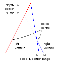
Most conventional stereo algorithms contain a fixed limit on the size of the epipolar search bands to use, this constrains the algorithm to always search between fixed disparity limits (and consequently over a fixed depth range in a scene, see Figure 2 below). Such constraints will usually be applied because the data in the scene is known to exist over a limited range of depths. Therefore, hand-tuning the algorithm's search parameters is often sufficient to perform successfully stereo matching. Obviously such manual intervention is undesirable for an autonomous vision system which will be expected to cope with a wide variety of scenes.

Figure 2, The direct relationship between epipolar search band size and the expected depths of objects/features in a scene.
Alternatively, stereo algorithms can perform a exhaustive searches over the entire disparity range present in the image (the only limit being; disparity > 0, because points cannot lie behind the camera) which avoids the trap of implicitly constraining the scene data to only exist over a limited fixed depth range. However, exhaustive search bands can introduce large amounts of ambiguity into the correspondence problem unless the scene is one in which ambiguity is not going to play a large problem (e.g. when using controlled/structured lighting).
In [3], the probability of an incorrect stereo match was show to be:
![]()
Where ![]() is
the is the probability of mismatching a pair of features when neither feature
has its correct match detected in the other image,
is
the is the probability of mismatching a pair of features when neither feature
has its correct match detected in the other image, ![]() is
the probability of mismatch when one feature has had its correct match
detected, and
is
the probability of mismatch when one feature has had its correct match
detected, and ![]() is
the probability of mismatch when both features have had their correct matches
found in the other image. Each of
is
the probability of mismatch when both features have had their correct matches
found in the other image. Each of ![]() ,
,
![]() ,
and
,
and ![]() are
proportional to the mean number of candidate matches and thus
are
proportional to the mean number of candidate matches and thus ![]() is
proportional to the epipolar area searched during matching.
is
proportional to the epipolar area searched during matching.
The previous section shows that for any given stereo matching algorithm we can minimise the probability of mismatch by reducing the search area. However, in the absence of information regarding the range of expected disparities, a suitable minimum search area and location cannot be established. One way to acquire this information is to encapsulate the matching algorithm within a temporal loop where disparities from the previous frame are used to seed matching in the current frame. In this way the search ranges can be kept as small as possible with the matching algorithm being used to track disparities from frame to frame, thus reducing the probability of a mismatch. [1, 2] achieve this by searching in the range along an epi-polar based on the disparities recovered from a local neighbourhood surrounding the current correlation block.
In [2], the success of the disparity bootstrapping for wide baseline
correlation stereo is demonstrated. (Although the stereo algorithm is described
as correlation based, for accuracy, the correlation metric was actually
used as a means to matching edge features.) By keeping the size of the
epipolar search bands to a minimum, the stereo mismatch probability, ![]() ,
is kept to a minimum, and the amount of outliers (incorrectly matched stereo
features) present in the output 3-D data is reduced when compared with
an exhaustive search algorithm.
,
is kept to a minimum, and the amount of outliers (incorrectly matched stereo
features) present in the output 3-D data is reduced when compared with
an exhaustive search algorithm.
Because the temporal stereo algorithm is using directed controlled epipolar seaches, the computational load required to process a single stereo image pair is reduced. Given the mutually supporting facts that reduced search range leads to increased robustness and a reduced computation load allow a temporal algorithm to process more frames per second than a standard stereo algorithm, this would seem to make these type of algorithms ideal for suggested applications mentioned above.
Coarse-to-Fine Bootstrapping for Temporal Stereo
Algorithms such as [5] and the temporal correlation stereo technique mentioned above, both suffer from start-up problems. [2] demonstrates that, on start-up, temporal stereo, like simulated annealing algorithms, can get stuck in local minima in the correlation search space, leading to outliers in the 3-D data. When there is sufficient motion in the scene, [2] did demonstrate that temporal stereo is able to converge on the correct solution, however the more typical approach is to assume that there is an accurate initial set of stereo correspondences for the scene available at algorithm start-up.
In [1], the issue of start-up problems for temporal stereo is addressed. The suggested solution; a coarse-to-fine (CTF) approach is selected as an ideal bootstrap method because it can integrate well with the existing temporal stereo algorithm (the image coarsening being done simultaneously with the preprocessing image rectification stage), and the effectiveness of the CTF approach for conventional stereo has already been demonstrated several times [16, 17]. In order to achieve the initial exhaustive search that is required to give a temporal stereo algorithm a good seed point from which to start, the early frames in a stereo sequence can be subjected to an additional CTF image pre-processing stage. Processing the initial few frames at a coarser scale (for example 30% to 50% of their original size) allows a correlation stereo algorithm to perform much larger epipolar band searches, but without increasing the computational load per frame. The CTF scale is then increased with each successive frame until the 100% image size is reached, and the temporal algorithm can proceed as normal. Hence the temporal stereo algorithm suffers no extra computational loading due to iterative constraints because each stereo image pair is only processed once, at a single CTF scale.
The benefit of this approach is that a valid 3D result is available from the first frame, and, the analysis in [1] demonstrates the fact that the result is more robust to outliers than the original temporal result processed at 100% image size.
Temporal Correlation Stereo: Example Results
|
Artificial Images (note: results show 3-D results data in black, superimposed on ground truth data in grey) |
AVI Movies |
Comments |
|
Artificial Cubes Sequence |
|
A sequence of 8 stereo frames rendered using the POV-Ray ray tracing package. |
|
Conventional Stereo Result |
|
The conventional stereo result contains numerous outliers as a consequence of having to use large epipolar search bands. |
|
Temporal Stereo Result (sequence start-up period) |
|
The temporal result quickly converges on robust 3-D data from having no initial data on scene structure although the first few results do contain outliers. |
|
Temporal Stereo Result (post start-up period) |
|
The temporal stereo algorithm is able to deliver robust 3-D data as the scene structure changes over time once the whole scene structure is known. |
|
Temporal Stereo with Coarse-to-Fine Bootstrap (sequence start-up period) |
|
The coarse-to-fine bootstrap allows the stereo algorithm to produce robust data from the very first frame. The result is refined using finer scales over time so the temporal result converges on an accurate and robust representation of the scene. |
|
Real Images |
AVI Movies |
Comments |
|
Real Cubes Sequence |
|
A sequence of 8 stereo frames of 3 real moving cube objects. |
|
Temporal Stereo with Coarse-to-Fine Bootstrap (sequence start-up period) |
|
The coarse-to-fine bootstrap allows the stereo algorithm to produce robust data from the very first frame. The result is refined using finer scales over time so the temporal result converges on an accurate and robust representation of the scene. |
Bibliography