|
|
Geometric vision is an important and well-studied part of computer vision. A wealth of useful results has been achieved in the last 15 years and has been reported in comprehensive monographies, e.g., [4, 12, 6], a sign of maturity for a research subject.
It is worth reminding the reader that geometry is an important but not the only important aspect of computer vision, and in particular of multi-view vision. The information brought by each image pixel is twofold: its position and its colour (or brightness, for a monochrome image). Ultimately, each computer vision system must start with brightness values, and, to smaller or greater depth, link such values to the 3D world.
|
|
The ambient space is modellled as a projective 3-D space  3, obtained by
completing the affine space
3, obtained by
completing the affine space  3 with a projective plane, known as plane at
infinity
3 with a projective plane, known as plane at
infinity 
 . In this ideal plane lie the intersections of the planes parallel in
X3.
. In this ideal plane lie the intersections of the planes parallel in
X3.
The projective coordinates of a point in 3 are 4-tuples defined up to a scale
factor. We write
 | (1) |
where  indicates equality to within a multiplicative factor.
is defined by its equation t = 0.
The points of the affine space are those of 3 which do not belong to .
Their projective coordinates are thus of the form (x,y,z, 1), where (x,y,z) are the
usual affine coordinates.
The linear transformations of a projective space into itself are called
collineations or homographies. Any collineation of 3 is represented by a generic
4 × 4 invertible matrix.
Affine transformations of 3 are the subgroup of collineations of 3 that
preserves the plane at infinity.
Similarity transformations are the subgroup of affine transformations of 3
that leave invariant a very special curve, the absolute conic, which is in the plane
at infinity and whose equation is:
 | (2) |
The space is therefore stratified into more and more specialized structures:
The stratification reflects the amount of knowledge that we possess about the scene and the sensor.
The pin-hole camera is described by its optical centre C (also known as camera projection centre) and the image plane.
The distance of the image plane from C is the focal length f.
The line from the camera centre perpendicular to the image plane is called the principal axis or optical axis of the camera.
The plane parallel to the image plane containing the optical centre is called the principal plane or focal plane of the camera.
The relationship between the 3D coordinates of a scene point and the coordinates of its projection onto the image plane is described by the central or perspective projection.
A 3D point is projected onto the image plane with the line containing the point and the optical centre (see Figure 2).
Let the centre of projection be the origin of a Euclidean coordinate system wherein the z-axis is the principal axis.
By similar triangles it is readily seen that the 3D point (x,y,z)T is mapped to the point (fx/z,fy/z)T on the image plane.
If the world and image points are represented by homogeneous vectors, then perspective projection can be expressed in terms of matrix multiplication as
 | (3) |
The matrix describing the mapping is called the camera projection matrix P.
Equation (3) can be written simply as:
 | (4) |
where M = (x,y,z, 1)T are the homogeneous coordinates of the 3D point and m = (fx/z,fy/z, 1)T are the homogeneous coordinates of the image point.
The projection matrix P in Equation (3) represents the simplest possible case, as it only contains information about the focal distance f.
General camera: bottom up approach The above formulation assumes a special choice of world coordinate system and image coordinate system. It can be generalized by introducing suitable changes of the coordinates systems.
Changing coordinates in space is equivalent to multiplying the matrix P to the right by a 4 × 4 matrix:
![[ ]
R t
G = 0 1](tutorial5x.gif) | (5) |
G is composed by a rotation matrix R and a translation vector t. It describes the position and orientation of the camera with respect to an external (world) coordinate system. It depends on six parameters, called external parameters.
The rows of R are unit vectors that, together with the optical centre, define the camera reference frame, expressed in world coordinates.
Changing coordinates in the image plane is equivalent to multiplying the matrix P to the left by a 3 × 3 matrix:
 | (6) |
K is the camera calibration matrix; it encodes the transformation from image coordinates to pixel coordinates in the image plane.
It depends on the so-called intrinsic parameters:
 between the axes (usually
  /2).
/2).The ratio sy/sx is the aspect ratio (usually close to 1).
Thus the camera matrix, in general, is the product of three matrices:
![P = K[I |0]G = K[R |t]](tutorial7x.gif) | (7) |
In general, the projection equation writes:
 | (8) |
where  is the distance of M from the focal plane of the camera (this will be
shown after), and m = (u,v, 1)T .
is the distance of M from the focal plane of the camera (this will be
shown after), and m = (u,v, 1)T .
Note that, except for a very special choice of the world reference frame, this “depth” does not coincide with the third coordinate of M.
General camera: top down approach
If P describes a camera, also  P for any 0 /=
 describes the same camera,
since these give the same image point for each scene point.
describes the same camera,
since these give the same image point for each scene point.
In this case we can also write:
 | (9) |
where means “equal up to a scale factor.”
In general, the camera projection matrix is a 3 × 4 full-rank matrix and, being homogeneous, it has 11 degrees of freedom.
Using QR factorization, it can be shown that any 3 × 4 full rank matrix P can be factorised as:
![P = cK[R |t],](tutorial10x.gif) | (10) |
( is defined because K(3, 3) = 1).
Projection centre The camera projection centre C is the only point for which the projection is not defined, i.e.:
 | (11) |
where  is a three-vector containing the affine (non-homogeneous) coordinates of
the optical centre.
is a three-vector containing the affine (non-homogeneous) coordinates of
the optical centre.
After solving for  we obtain:
 | (12) |
where the matrix P is represented by the block form: P = [P3×3|p4] (P3×3 is the matrix composed by the first three rows and first three columns of P, and p4 is the fourth column of P).
A few words about normalization
If = 1 in Eq. (10), the matrix P is said to be normalized.
If (and only if) the matrix is normalized, then in the projection equation (8)
is the distance of M from the focal plane of the camera (usually referred to as
depth).
We observe that:
 | (13) |
In particular, the third component is = p3T ( -
- ), where p
3T is the third row
of P3×3.
), where p
3T is the third row
of P3×3.
If write R in terms of its rows and multiply in Eq. (7) we see that p3T is the third row of R, which correspond to the versor of the principal axis.
Hence, the previous equations says that is the projection of the vector
( -
- ) onto the principal axis, i.e., the depth of M.
In general (when the camera is not normalized), contains an arbitrary scale
factor. Can we recover this scale factor from a generic camera matrix P without
factorizing it like in Eq. (10)?
We only need to observe that if P is given by Eq. (10), p3T is the third row of
R multiplied by the scale factor . Hence, = ||p3||.
Optical ray The projection can be geometrically modelled by a ray through the optical centre and the point in space that is being projected onto the image plane (see Fig. 2).
The optical ray of an image point m is the locus of points in space that projects onto m.
It can be described as a parametric line passing through the camera projection centre C and a special point (at infinity) that projects onto m:
 | (14) |
Please note that, provided that P is normalized, the parameter in the
equation of the optical ray correspond to the depth of the point M.
We will prove now that the image of the absolute conic depends on the intrinsic parameters only (it is unaffected by camera position and orientation).
The points in the plane at infinity have the form M = ( T , 0)T , hence
T = KR ~M.](tutorial22x.gif) | (15) |
The image of points on the plane at infinity does not depend on camera position (it is unaffected by camera translation).
The absolute conic (which is in the plane at infinity) has equation  T
T  = 0,
therefore its projection has equation:
= 0,
therefore its projection has equation:
 | (16) |
The conic  = (KK-T )-1 is the image of the absolute conic.
The angle (a metrical property) between two rays is determined by the image of the absolute conic.
Let us consider a camera P = [K|0], then m =  K
K . Let be the angle
between the rays trough M1 and M1, then
. Let be the angle
between the rays trough M1 and M1, then
 | (17) |
A number of point correspondences mi  Mi is given, and we are required to find
a camera matrix P such that
Mi is given, and we are required to find
a camera matrix P such that
 | (18) |
The equation can be rewritten in terms of the cross product as
 | (19) |
This form will enable a simple a simple linear solution for P to be derived. Using
the properties of the Kronecker product ( ) and the vec operator, we
derive:
) and the vec operator, we
derive:
![mi × PMi = 0 <====> [mi]× P Mi = 0 <====> vec([mi] ×P Mi) = 0 <====>
<====> (MT ox [m ] ) vecP = 0 <====> ([m ] ox MT )vecP T = 0
i i× i× i](tutorial32x.gif)
 | (20) |
Although there are three equations, only two of them are linearly independent: we can write the third row (e.g.) as a linear combination of the first two.
From a set of n point correspondences, we obtain a 2n × 12 coefficient matrix A by stacking up two equations for each correspondence.
In general A will have rank 11 (provided that the points are not all coplanar) and the solution is the 1-dimensional right null-space of A.
The projection matrix P is computed by solving the resulting linear system of equations, for n > 6.
If the data are not exact (noise is generally present) the rank of A will be 12 and a least-squares solution is sought.
The least-squares solution for vec PT is the singular vector corresponding to the smallest singular value of A.
This is called the Direct Linear Transform (DLT) algorithm [12].
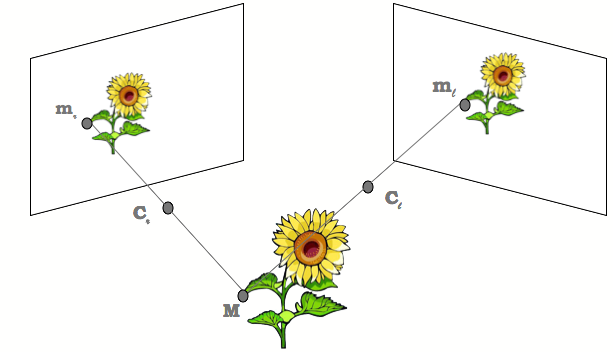
The two-view geometry is the intrinsic geometry of two different perspective views of the same 3D scene (see Figure 4). It is usually referred to as epipolar geometry.
The two perspective views may be acquired simultaneously, for example in a stereo rig, or sequentially, for example by a moving camera. From the geometric viewpoint, the two situations are equivalent, but notice that the scene might change between successive snapshots.
Most 3D scene points must be visible in both views simultaneously. This is not
true in case of occlusions, i.e., points visible only in one camera. Any
unoccluded 3D scene point M = (x,y,z, 1)T is projected to the left and right
view as m = (u,v, 1)T and m
r = (ur,vr, 1)T , respectively (see Figure
4).
= (u,v, 1)T and m
r = (ur,vr, 1)T , respectively (see Figure
4).
Image points m and mr are called corresponding points (or conjugate points)
as they represent projections of the same 3D scene point M.
The knowledge of image correspondences enables scene reconstruction from images.
|
|
Algebraically, each perspective view has an associated 3 × 4 camera projection
matrix P which represents the mapping between the 3D world and a 2D image.
We will refer to the camera projection matrix of the left view as P and of the
right view as Pr. The 3D point M is then imaged as (21) in the left view, and
(22) in the right view:
 | (21) |
 | (22) |
Geometrically, the position of the image point m in the left image
plane I can be found by drawing the optical ray through the left camera
projection centre C and the scene point M. The ray intersects the left
image plane I at m. Similarly, the optical ray connecting Cr and M
intersects the right image plane Ir at mr. The relationship between image
points m and mr is given by the epipolar geometry, described in Section
4.1.
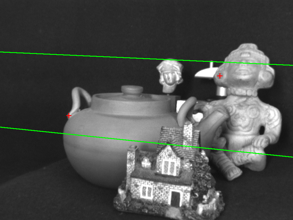
The epipolar geometry describes the geometric relationship between two perspective views of the same 3D scene.
The key finding, discussed below, is that corresponding image points must lie on particular image lines, which can be computed without information on the calibration of the cameras.
This implies that, given a point in one image, one can search the corresponding point in the other along a line and not in a 2D region, a significant reduction in complexity.
Any 3D point M and the camera projection centres C and Cr define a plane
that is called epipolar plane.
The projections of the point M, image points m and mr, also lie in the
epipolar plane since they lie on the rays connecting the corresponding camera
projection centre and point M.
The conjugate epipolar lines, l and lr, are the intersections of the epipolar
plane with the image planes. The line connecting the camera projection centres
(C,Cr) is called the baseline.
The baseline intersects each image plane in a point called epipole.
By construction, the left epipole e is the image of the right camera
projection centre Cr in the left image plane. Similarly, the right epipole er
is the image of the left camera projection centre C in the right image
plane.
All epipolar lines in the left image go through e and all epipolar lines in the
right image go through er.
The epipolar constraint. An epipolar plane is completely defined by the camera projection centres and one image point.
Therefore, given a point m, one can determine the epipolar line in the right
image on which the corresponding point, mr, must lie.
The equation of the epipolar line can be derived from the equation
describing the optical ray. As we mentioned before, the right epipolar line
corresponding to m geometrically represents the projection (Equation
(8)) of the optical ray through m (Equation (14)) onto the right image
plane:
 | (23) |
If we now simplify the above equation we obtain the description of the right epipolar line:
 | (24) |
This is the equation of a line through the right epipole er and the image point
m' = P3×3,rP3×3,l-1m
which represents the projection onto the right image
plane of the point at infinity of the optical ray of m.
The equation for the left epipolar line is obtained in a similar way.
The epipolar geometry can be described analytically in several ways, depending on the amount of the a priori knowledge about the stereo system. We can identify three general cases.
If both intrinsic and extrinsic camera parameters are known, we can describe the epipolar geometry in terms of the projection matrices (Equation (24)).
If only the intrinsic parameters are known, we work in normalised coordinates and the epipolar geometry is described by the essential matrix.
If neither intrinsic nor extrinsic parameters are known the epipolar geometry is described by the fundamental matrix.
If the intrinsic parameters are known, we can switch to normalised coordinates:
m  K-1m (please note that this change of notation will hold throughout this
section).
K-1m (please note that this change of notation will hold throughout this
section).
Consider a pair of normalised cameras. Without loss of generality, we can fix the world reference frame onto the first camera, hence:
![Pl = [I|0] and Pr = [R |t].](tutorial39x.gif) | (25) |
With this choice, the unknown extrinsic parameters have been made explicit.
If we substitute these two particular instances of the camera projection matrices in Equation (24), we get
 | (26) |
in other words, the point mr lies on the line through the points t and Rm. In
homogeneous coordinates, this can be written as follows:
 | (27) |
as the homogeneous line through two points is expressed as their cross product.
Similarly, a dot product of a point and a line is zero if the point lies on the line.
The cross product of two vectors can be written as a product of a skew-symmetric matrix and a vector. Equation (27) can therefore be equivalently written as
![mTr [t]× Rml = 0,](tutorial42x.gif) | (28) |
where [t]× is the skew-symmetric matrix of the vector t. If we multiply the
matrices in the above equation, we obtain a single matrix which describes the
relationship between the corresponding image points m and mr in normalised
coordinates. This matrix is called the essential matrix E:
![E = [t]×R,](tutorial43x.gif) | (29) |
and the relationship between two corresponding image points in normalised coordinates is expressed by the defining equation for the essential matrix:
 | (30) |
E encodes only information on the extrinsic camera parameters. It is singular, since det[t]× = 0. The essential matrix is a homogeneous quantity. It has only five degrees of freedom: a 3D rotation and a 3D translation direction.
The fundamental matrix can be derived in a similar way to the essential matrix. All camera parameters are assumed unknown; we write therefore a general version of Equation (25):
![Pl = Kl[I|0] and Pr = Kr[R |t].](tutorial45x.gif) | (31) |
Inserting these two projection matrices into Equation (24), we get
 | (32) |
which states that point mr lies on the line through er and KrRK-1m
. As in the
case of the essential matrix, this can be written in homogeneous coordinates
as:
![mTr [er]× KrRK -l 1ml = 0.](tutorial47x.gif) | (33) |
The matrix
![F = [er]×KrRK -l1](tutorial48x.gif) | (34) |
is the fundamental matrix F, giving the relationship between the corresponding image points in pixel coordinates.
The defining equation for the fundamental matrix is therefore
 | (35) |
F is the algebraic representation of the epipolar geometry. It is a 3 × 3, rank-two homogeneous matrix. It has only seven degrees of freedom since it is defined up to a scale and its determinant is zero. Notice that F is completely defined by pixel correspondences only (the intrinsic parameters are not needed).
For any point m in the left image, the corresponding epipolar line lr in the
right image can be expressed as
 | (36) |
Similarly, the epipolar line l in the left image for the point mr in the right image
can be expressed as
 | (37) |
The left epipole e is the right null-vector of the fundamental matrix
and the right epipole is the left null-vector of the fundamental matrix:
One can see from the derivation that the essential and fundamental
matrices are related through the camera calibration matrices K and
Kr:
 | (40) |
Consider a camera pair. Using the fact that if F maps points in the left image to epipolar lines in the right image, then FT maps points in the right image to epipolar lines in the left image, Equation (32) gives:
 | (41) |
This is another way of writing the epipolar constraint: the epipolar line of mr
(FT m
r) is the line containing its corresponding point (m) and the epipole in the
left image (e).
If a number of point correspondences mi m
ri is given, we can use Equation
(35) to compute the unknown matrix F.
We need to convert Equation (35) from its bilinear form to a form that matches the null-space problem, as in the DLT algorithm. To this end we introduce the vec operator1:

Each point correspondence gives rise to one linear equation in the unknown entries of F. From a set of n point correspondences, we obtain a n × 9 coefficient matrix A by stacking up one equation for each correspondence.
In general A will have rank 8 and the solution is the 1-dimensional right null-space of A.
The fundamental matrix F is computed by solving the resulting linear system of equations, for n > 8.
If the data are not exact and more than 8 points are used, the rank of A will be 9 and a least-squares solution is sought.
The least-squares solution for vec F is the singular vector corresponding to the smallest singular value of A.
This method does not explicitly enforce F to be singular, so it must be done a posteriori.
Replace F by F' such that det F' = 0, by forcing to zero the least singular value.
It can be shown that F' is the closest singular matrix to F in Frobenius norm.
Geometrically, the singularity constraint ensures that the epipolar lines meet in a common epipole.
Given the camera matrices P and Pr, let m and mr be two corresponding points
satisfying the epipolar constraint mrT Fm
= 0. It follows that mr lies on the
epipolar line Fm and so the two rays back-projected from image points m and
mr lie in a common epipolar plane. Since they lie in the same plane, they will
intersect at some point. This point is the reconstructed 3D scene point
M.
Analytically, the reconstructed 3D point M can be found by solving for
parameter or r in Eq. (24). Let us rewrite it as:
 | (42) |
The depth r and are unknown. Both encode the position of M in space, as r
is the depth of M wrt the right camera and is the depth of M wrt the left
camera.
The three points mr,er and m' are known and are collinear, so we can solve
for using the following closed form expressions [41]:
 | (43) |
The reconstructed point M can then be calculated by inserting the value into
Equation (14).
In reality, camera parameters and image locations are known only approximately. The back-projected rays therefore do not actually intersect in space. It can be shown, however, that Formula (43) solve Eq. (42) in a least squares sense [26].
Triangulation is addressed in more details in [2, 15, 12, 51].
When observing a plane, we obtain an interesting specialization of the epipolar geometry of two views.
First, let us establish that the map between a world plane and its
perspective image is a collineation of 2. The easiest way to see it is to
choose the world coordinate system such that the plane has equation
z = 0.
Expanding the projection erquation gives:
 | (44) |
Points are mapped from the world plane to the image plane with a 3 × 3
non-singular matrix, which represents a collineation of 2.
Next, we prove that: images of points on a plane are related to corresponding
image points in a second view by a collineation (or homography) of 2.
We have one collineation from to the left image plane, and another
collineation from to the right image plane. By composing the inverse of the first
with the second, we define a collineation from the image plane of the left camera
to the image plane of the right camera.
The plane induces a collineation H between the views, which transfers
points from one view to the other:
between the views, which transfers
points from one view to the other:
 | (45) |
where H is a 3 × 3 non-singular matrix.
Even though a collineation of 2 depends upon eight parameters, there is no
contradiction with the fact that a plane depends upon three parameters. Indeed,
the collineation induced by a plane must be compatible with the epipolar
geometry, i.e.:
 | (46) |
for all points m. This implies that the matrix HT F is antisymmetric:
 | (47) |
and this imposes six homogeneous constraints on H.
A collineation H that satisfies Eq. (47) is said to be compatible with F.
A collineation H is compatible with F if and only if
![F -~ [er]× H](tutorial63x.gif) | (48) |
From the latter follows that - provided that does not contain Cr
-
 | (49) |
If the 3D point M lies on a plane with equation nT M = d, Eq. (32) can be
specialized, obtaining (after elaborating):
 | (50) |
Therefore, the collineation induced by is given by:
 | (51) |
This is a three-parameter family of collineations, parameterized by n/d.
The infinite homography H is the collineation induced by the plane at infinity;
it maps vanishing points to vanishing points (a vanishing point is where all the
lines that shares the same direction meet).
It can be derived by letting d 
 in (50), thereby obtaining:
 | (52) |
The infinity homography does not depend on the translation between views.
Note that H can be obtained if t = 0 in Eq. (32), which corresponds to a
rotation about the camera centre. Thus H not only relates points at infinity
when the camera describes a general motion, but it also relates image points of
any depth if the camera rotates about its centre.
In general, when points are not on the plane, the homography induced by a plane generates a virtual parallax. This gives rise to an alternative representation of the epipolar geometry and scene structure [43].
First, let us note that Eq. (32), which we write
 | (53) |
can be seen as composed by a transfer with the infinity homography (Hm) plus
a parallax correction term ( er).
er).
We want to generalize this equation to any plane. To this end we substitute
 | (54) |
into Eq. (53), obtaining
 | (55) |
with  =
=  , where a is the distance of M to the plane .
When M is on the 3D plane , then mr Hm. Otherwise there is a residual
displacement, called parallax, which is proportional to and oriented along the
epipolar line.
The magnitude parallax depends only on the left view and the plane. It does not depend on the parameters of the right view.
From Eq. (55) we derive mrT (e
r × Hm) = 0, hence
![F -~ [er]×HTT](tutorial74x.gif) | (56) |
|
|
A number of point correspondences mri m
i is given, and we are required to
find an homography matrix H such that
 | (57) |
The equation (we drop the index i for simplicity) can be rewritten in terms of the cross product as
 | (58) |
As we did before, we exploit the properties of the Kronecker product and the vec operator to transform this into a null-space problem and then derive a linear solution:
![mr × Hml = 0 <====> [mr] ×Hml = 0 <====> vec([mr] ×Hml) = 0
<====> (mT ox [m ] )vec H = 0 <====> ([m ] ox mT ) vecHT = 0
l r × r × l](tutorial80x.gif)
 | (59) |
Although there are three equations, only two of them are linearly independent: we can write the third row (e.g.) as a linear combination of the first two.
From a set of n point correspondences, we obtain a 2n× 9 coefficient matrix A by stacking up two equations for each correspondence.
In general A will have rank 8 and the solution is the 1-dimensional right null-space of A.
The projection matrix H is computed by solving the resulting linear system of equations, for n > 4.
If the data are not exact, and more than 4 points are used, the rank of A will be 9 and a least-squares solution is sought.
The least-squares solution for vec HT is the singular vector corresponding to the smallest singular value of A.
This is another incarnation of the DLT algorithm.
The epipole can be located [48] given the homography H between two
views and two off-plane conjugate pairs m0 m
r0 and m
1 m
r1
.
|
 |
Following simple geometric consideration, the epipole is computed as the
intersection between the line containing Hm0,m
r0 and the line containing
Hm1,m
r1:
 | (60) |
In the projective plane, the line determined by two points is given by their cross product, as well as the point determined by two lines.
We are required to compute the magnitude of the parallax for a point m given
its corresponding point mr, the homography H between the two views and the
epipole. To this end we rewrite (55) as:
 | (61) |
and, given that points er, mr and Hm are collinear, we solve for
using:
 | (62) |
Please note that the epipole and the homography can be computed from images only up to an unknown scale factor. It follows that the magnitude of the parallax as well is known only up to a scale factor.
Mosaics. Image mosaicing is the automatic alignment (or registration) of multiple images into larger aggregates [46]. There are two types of mosaics. In both cases, it turns out that images are related by homographies, as we discussed previously.
|
    
|
Orthogonal rectification. The map between a world plane and its perspective image is an homography. The world-plane to image-plane homography is fully defined by four points of which we know the relative position in the world plane. Once this homography is determined, the image can be back projected (warped) onto the world plane. This is equivalent to synthesize an image as taken from a fronto-parallel view of the plane. This is known as orthogonal rectification [29] of a perspective image.
What can be reconstructed depends on what is known about the scene and the stereo system. We can identify three cases.
If only intrinsics are known (plus point correspondences between images), the epipolar geometry is described by the essential matrix (Section 4.1.1). We will see that, starting from the essential matrix, only a reconstruction up to a similarity transformation (rigid+ uniform scale) can be achieved. Such a reconstruction is referred to as “Euclidean”.
Unlike the fundamental matrix, the only property of which is to have rank two, the essential matrix is characterised by the following theorem [22].
Theorem 4.1 A real 3 × 3 matrix E can be factorised as product of a nonzero skew-symmetric matrix and a rotation matrix if and only if E has two identical singular values and a zero singular value.
The theorem has a constructive proof (see [13]) that describes how E can be factorised into rotation and translation using its Singular Value Decomposition (SVD).
The rotation R and translation t are then used to instantiate a camera pair as in Equation (25), and this camera pair is subsequently used to reconstruct the structure of the scene by triangulation.
The rigid displacement ambiguity arises from the arbitrary choice of the world reference frame, whereas the scale ambiguity derives from the fact that t can be scaled arbitrarily in Equation (29) and one would get the same essential matrix (E is defined up to a scale factor).
Therefore translation can be recovered from E only up to an unknown scale factor which is inherited by the reconstruction. This is also known as depth-speed ambiguity.
Suppose that a set of image correspondences mi m
ri are given. It is assumed
that these correspondences come from a set of 3D points Mi, which are unknown.
Similarly, the position, orientation and calibration of the cameras are not known.
This situation is usually referred to as weak calibration, and we will see that the
scene may be reconstructed up to a projective ambiguity, which may
be reduced if additional information is supplied on the cameras or the
scene.
The reconstruction task is to find the camera matrices P and Pr, as well as
the 3D points Mi such that
 | (63) |
If T is any 4 × 4 invertible matrix, representing a collineation of 3, then
replacing points Mi by TMi and matrices P
and Pr by PT-1 and P
rT-1 does
not change the image points mi. This shows that, if nothing is known but the
image points, the structure Mi and the cameras can be determined only up to a
projective transformation.
The procedure for reconstruction follows the previous one. Given the weak calibration assumption, the fundamental matrix can be computed (using the algorithm described in Section 4.1.2), and from a (non-unique) factorization of F of the form
![F = [er]×A](tutorial94x.gif) | (64) |
two camera matrices P and Pr:
![Pl = [I|0] and Pr = [A |er],](tutorial95x.gif) | (65) |
can be created in such a way that they yield the fundamental matrix F, as can be easily verified. The position in space of the points Mi is then obtained by triangulation.
The only difference with the previous case is that F does not admit a unique factorization, whence the projective ambiguity follows.
Indeed, for any A satisfying Equation (64), also A + erxT for any vector x, satisfies Equation (64).
One matrix A satisfying Equation (64) can be obtained as A = -[er]×F (this is called the epipolar projection matrix [31]).
More in general, any homography induced by a plane can be taken as the A matrix (cfr. Eq. (48)).
In this section we study the relationship that links three or more views of the same 3D scene, known in the three-view case as trifocal geometry.
This geometry can be described in terms of fundamental matrices linking pairs of cameras, but in the three-view case a more compact and elegant description is provided by a special algebraic operator, the trifocal tensor.
We also discover that three views are all we need, in the sense that additional views do not allow us to compute anything we could not already compute (Section 5.4).
Denoting the cameras by 1, 2, 3, there are now three fundamental matrices, F1,2, F1,3, F2,3, and six epipoles, ei,j, as in Figure 13. The three fundamental matrices describe completely the trifocal geometry [7].
The plane containing the three optical centres is called the trifocal plane. It intersects each image plane along a line which contains the two epipoles.
Writing Eq. (41) for each camera pair (taking the centre of the third camera as the point M) results in three epipolar constraints:
 | (66) |
Three fundamental matrices include 21 free parameters, less the 3 constraints above; the trifocal geometry is therefore determined by 18 parameters.
This description of the trifocal geometry fails when the three cameras are collinear, and the trifocal plane reduces to a line.
Point transfer If the trifocal geometry is known, given two conjugate points m1 and m2 in view 1 and 2 respectively, the position of the conjugate point m3 in view 3 is completely determined (Figure 14).
This allows for point transfer or prediction. Indeed, m3 belongs simultaneously to the epipolar line of m1 and to the epipolar line of m2, hence:
 | (67) |
View synthesis [27, 1, 3], exploit the trifocal geometry to generate novel (synthetic) images starting from two reference views. A related topic is image-based rendering [28, 52, 24].
Epipolar transfer fails when the three optical rays are coplanar, because the epipolar lines are coincident. This happens:
These deficiencies motivate the introduction of an independent trifocal constraint.
Recalling Equation (65), consider the following three cameras:
![P1 = [I| 0], P2 = [A2 |e2,1], and P3 = [A3|e3,1].](tutorial100x.gif) | (68) |
Consider a point M in space projecting to m1, m2 and m3 in the three cameras. Let us write the epipolar line of m1 in the other two views (using Equation (24)):
| 2m2 | = e2,1 + 1A2m1 | (69) |
| 3m3 | = e3,1 + 1A3m1. | (70) |
Consider a line through m2, represented by s2; we have s2T m 2 = 0, that substituted in (69) gives:
 | (71) |
Likewise, for a line through m3 represented by s3 we can write:
 | (72) |
After eliminating 1 from Equation (71) and (72) we obtain:
 | (73) |
and after some re-writing:
 | (74) |
This is the fundamental trifocal constraint, that links (via a trilinear equation) m1, s2 (any line through m2) and s3 (any line through m3).
Geometrically, the trifocal constraint imposes that the optical rays of m1 intersect the 3D line L that projects onto s2 in the second image and s3 in the third image.
Please note that given two (arbitrary) lines in two images, they can be always seen as the image of a 3D line L, because two planes always define a line, in projective space (this is why there is no such thing as the epipolar constraint between lines.)
The trifocal constraint represents the trifocal geometry (nearly) without singularities. It only fails is when the cameras are collinear and the 3D point is on the same line.
|
We can write this trilinear form (Eq. (74)) as2:


Using the vec-transpose operator [38], Eq. (74) can be also re-written as:
 | (75) |
where (Tm1)(3) is a 3 × 3 matrix such that vec(Tm 1)(3) = Tm 1.
Trifocal constraints for points. Since a point is determined by two lines, we can write a similar independent constraint for a second line. Such two lines determining a point m are represented by any two rows of [m]×. To keep notation compact let us consider the whole matrix [m]×. The trifocal constraints for three points writes:
![[m2] ×(T m1)(3)[m3] × = 0.](tutorial109x.gif) | (76) |
This is a matrix equation which gives 9 scalar equations, only four of which are independent. Equivalently
![(mT1 ox [m3] × ox [m2]× )vec(T) = 0](tutorial110x.gif) | (77) |
This equation can be used to recover T (likewise we did for F). The coefficient matrix is a 9 × 27 matrix of rank 4 (the rank of the Kronecker product is the product of the ranks), therefore every triplet (m1, m2, m3) of corresponding points gives four linear independent equations. Seven triplets determine the 27 entries of T.
Point transfer. Let s2T be a row of [m 2]×, then
![( )
sT2(Tm1)(3) [m3] × = 0](tutorial111x.gif) | (78) |
This implies that the transpose of the leftmost term in parentheses (which is a 3-vector) belongs to the kernel of [m3]×, which is equal to m3 (up to a scale factor) by construction. Hence
 | (79) |
This point transfer equation was derived by [39].
In this section we followed the approach of [39, 32] to avoid the tensorial notation. In the next slide, however, we will briefly sketch the tensorial interpretation of the trifocal constraint. A starting point to learn more on the trifocal tensor is [42].
The trifocal tensor. The trifocal tensor T is a a 3 × 3 × 3 array, which can be seen as a stack of three 3 × 3 matrices. The entries of T are those of the matrix T (just rearranged).
Indeed, (Tm1)(3) can be seen as the linear combination of 3 matrices with the components of m1:
![(T m1)(3) = ([t1|t2| t3]m1)(3) = (ut1 + vt2 + t3)(3) = ut(3)+ vt(3) + t(3)
1 2 3](tutorial113x.gif)
Therefore, the action of the tensor T (m1,s2,s3) = s2T (Tm 1)(3)s 3 is to first combine matrices of the stack according to m1, then combine the columns according to s3 and finally to combine the elements according to s2.
As in the case of two views, what can be reconstructed depends on what is known about the scene and the cameras.
If the internal parameters of the cameras are known, we can obtain a Euclidean reconstruction, that differs from the true reconstruction by a similarity transformation. This is composed by a rigid displacement (due to the arbitrary choice of the world reference frame) plus a a uniform change of scale (due to the well-known depth-speed ambiguity).
In the weakly calibrated case, i.e., when point correspondences are the only information available, a projective reconstruction can be obtained.
In both cases, the solution is not straightforward generalization of the two view case, as the problem of global consistency comes into play (i.e., how to relate each other the local reconstructions that can be obtained from view pairs).
Let us consider for simplicity the case of three views, which generalizes straightforward to N views.
If one applies the method of Section 4.4.1 to view pairs 1-2, 1-3 and 2-3 one
obtains three displacements (R12, 12), (R13,
 13) and (R23,
 23) known up a scale
factor, as the norm of translation cannot be recovered, (the symbol^indicates a
unit vector).
23) known up a scale
factor, as the norm of translation cannot be recovered, (the symbol^indicates a
unit vector).
The “true” displacements must satisfy the following compositional rule
 | (80) |
which can be rewritten as
 | (81) |
where  1 = ||t12||/||t13|| and 2 = ||t23||/||t13|| are unknown.
However, Eq. (80) constraints  13,R23
 12 and
  23 to be coplanar, hence the
ratios 1,2 can be recovered:
23 to be coplanar, hence the
ratios 1,2 can be recovered:
 | (82) |
And similarly for 2.
In this way three consistent camera matrices can be instantiated.
Note that only ratios of translation norm can be computed, hence the global scale factor remains undetermined.
If one applies the method of Section 4.4.2 to consecutive pairs of views, she would obtain, in general, a set of reconstructions linked to each other by an unknown projective transformation (because each camera pair defines its own projective frame).
An elegant method for multi-image reconstruction was described in [45], based on the same idea of the factorization method [47].
Consider m cameras P1...Pm looking at n 3D points M1...Mn. The usual projection equation
 | (83) |
can be written in matrix form:
![|_ 1 1 2 2 n n _| |_ _ |
z11m 11, z12m 12, ... z1nm 1n P1,
z2m 2, z2m 2, ... z2m 2 P , [ ]
... ... ... ... = 2. M1, M2, ... Mn .
1 1 2 2 n n |_ .. _| -------- --------
|_ zmm m, zmm m, ...zmm m _| Pm structure S
- -
------------ ------------ P
measurements W](tutorial124x.gif) | (84) |
In this formula the mij are known, but all the other quantities are unknown,
including the projective depths ij. Equation (84) tells us that W can be factored
into the product of a 3m× 4 matrix P and a 4 ×n matrix S. This also means that
W has rank four.
If we assume for a moment that the projective depths ij are known, then
matrix M is known too and we can compute its singular value decomposition:
 | (85) |
In the noise-free case, D = diag( 1,2,3,4, 0,...0), thus, only the first 4 columns
of U (V ) contribute to this matrix product. Let U3m×4 (V n×4) the matrix of the
first 4 columns of U (V ). Then:
1,2,3,4, 0,...0), thus, only the first 4 columns
of U (V ) contribute to this matrix product. Let U3m×4 (V n×4) the matrix of the
first 4 columns of U (V ). Then:
 | (86) |
The sought reconstruction is obtained by setting:
 | (87) |
For any non singular projective transformation T, TP and T-1S is an equally valid factorization of the data into projective motion and structure.
As expected, the reconstruction is up to an unknown projective transformation.
A consequence of this is that the choice of attaching the diagonal matrix to U3m×4 is arbitrary. It could be attached to V n×4 or even factorized in two matrices.
As the i,j are unknown, we are left with the problem of estimating them. The
original algorithm [45] uses the epipolar constraint (Eq.41) to fix the ratio of the
projective depths of one point in successive images.
In [17] the projective depths are estimated in an iterative fashion. First let us note that for a fixed camera i the projection equation writes:
![[ 1 2 n]
m i, m i, ... m i Zi = PiS](tutorial128x.gif) | (88) |
where Zi = diag(i,1,i,2,...i,n). The following iterative procedure is used:
i,j = 1;
5 is sufficiently small then stop;
It can be proven that the quantity that is being minimized is 5.
This technique is fast, requires no initialization, and gives good results in practice, although there is no guarantee that the iterative process will converge.
A provably convergent iterative method have been presented in [34].
We outline here an alternative and elegant way to derive all the meaningful multi-linear constraints on N views, based on determinants, described in [18]. Consider one image point viewed by m cameras:
 | (89) |
By stacking all these equations we obtain:
 | (90) |
This implies that the 3m × (m + 4) matrix (let us call it L) is rank-deficient, i.e., rank L < m + 4. In other words, all the (m + 4) × (m + 4) minors of L are equal to 0.
It has been proven that there are three different types of such minors that translates into meaningful multi-view constraints, depending on the number of rows taken from each view.
The minors that does not contain at least one row from each camera are identically zero, since they contain a zero column. Since one row has to be taken from each view and the remaining four can be distributed freely, one can choose:
All the other type of minors can be factorised as product of the two-, three-, or four-views constraints and point coordinates in the images3.
The aim of autocalibration is to compute the internal parameters, starting from weakly calibrated cameras.
More in general, the task is to recover metric properties of camera and/or scene, i.e., to compute a Euclidean reconstruction.
There are two classes of methods:
The reader is referred to [8] for a review of autocalibration, and to [35, 49, 21, 40, 37, 11] for classical and recent work on the subject.
Consider m cameras. The difference between the d.o.f. of the multifocal geometry (e.g. 7 for two views) and the d.o.f. of the rigid displacements (e.g. 5 for two views) is the number of independent constraints available for the computation of the intrinsic parameters (e.g. 2 for two views).
The multifocal geometry of m cameras (represented by the m-focal tensor) has
11m- 15 d.o.f. Proof: a set of m cameras have 11m d.o.f., but they determine the
m-focal geometry up to a collineation of 3, which has 15 d.o.f. The net sum is
11m - 15 d.o.f.
On the other hand, the rigid displacements in m views are described by 6m - 7 parameters: 3(m - 1) for rotations, 2(m - 1) for translations, and m - 2 ratios of translation norms.
Thus, m weakly calibrated views give 5m - 8 constraints available for computing the intrinsic parameters.
Let us suppose that mk parameters are known and mc parameters are constant.
The first view introduces 5 - mk unknowns. Every view but the first introduces 5 - mk - mc unknowns.
Therefore, the unknown intrinsic parameters can be computed provided that
 | (91) |
For example, if the intrinsic parameters are constant, three views are sufficient to recover them.
If one parameter (usually the skew) is known and the other parameters are varying, at least eight views are needed.
If we consider two views, two independent constraints are available for the computation of the intrinsic parameters from the fundamental matrix.
Indeed, F has 7 d.o.f, whereas E, which encode the rigid displacement, has only 5 d.o.f. There must be two additional constraint that E must satisfy, with respect to F.
In particular, these constraints stem from the equality of two singular values of the essential matrix (Theorem 4.1) which can be decomposed in two independent polynomial equations.
Let Fij be the (known) fundamental matrix relating views i and j, and let Ki and Kj be the respective (unknown) intrinsic parameter matrices.
The idea of [37] is that the matrix
 | (92) |
satisfies the constraints of Theorem 4.1 only if the intrinsic parameters are correct.
Hence, the cost function to be minimized is
 | (93) |
where 1
ij > 2
ij are the non zero singular values of Eij and wij are normalized
weight factors (linked to the reliability of the fundamental matrix estimate).
The previous counting argument shows that, in the general case of n views, the n(n - 1)/2 two-view constraints that can be derived are not independent, nevertheless they can be used as they over-determine the solution.
A non-linear least squares solution is obtained with an iterative algorithm (e.g. Gauss-Newton) that uses analytical derivatives of the cost function.
A starting guess is needed, but this cost function is less affected than others by local minima problems. A globally convergent algorithm based on this cost function is described in [9].
We have seen that a projective reconstruction can be computed starting from points correspondences only (weak calibration), without any knowledge of the camera matrices.
Projective reconstruction differs from Euclidean by an unknown projective transformation in the 3-D projective space, which can be seen as a suitable change of basis.
Starting from a projective reconstruction the problem is computing the transformation that “straighten” it, i.e., that upgrades it to an Euclidean reconstruction.
To this purpose the problem is stratified [31, 5] into different representations: depending on the amount of information and the constraints available, it can be analyzed at a projective, affine, or Euclidean level.
Let us assume that a projective reconstruction is available, that is a sequence Pi of m + 1 camera matrices and a set Mj of n + 1 3-D points such that:
 | (94) |
Without loss of generality, we can assume that camera matrices writes:
![P = [I |0]; P = [A |e ] for i = 1...m
0 i i i](tutorial135x.gif) | (95) |
We are looking for the a 4 × 4 nonsingular matrix T that upgrades the projective reconstruction to Euclidean:
 | (96) |
PiE = P iT is the Euclidean camera,
We can choose the first Euclidean-calibrated camera to be P0E = K 0[I | 0], thereby fixing arbitrarily the world reference frame:
![PE0 = K0[I |0] P Ei = Ki[Ri | ti] for i = 1 ...m.](tutorial137x.gif) | (97) |
With this choice, it is easy to see that P0E = P 0T implies
 | (98) |
where rT is a 3-vector and s is a scale factor, which we will arbitrarily set to 1 (the Euclidean reconstruction is up to a scale factor).
Under this parameterization T is clearly non singular, and it depends on eight parameters.
Substituting (98) in PiE P
iT gives
![P Ei = [KiRi |Kiti] - ~ PiT = [AiK0 + eirT| ei] for i > 0](tutorial139x.gif) | (99) |
and, considering only the leftmost 3 × 3 submatrix, gives
 | (100) |
Rotation can be eliminated using RRT = I, leaving:
 | (101) |
This is the basic equation for autocalibration (called absolute quadric constraint), relating the unknowns Ki (i = 0...m) and r to the available data Pi (obtained from weakly calibrated images).
Note that (101) contains five equations, because the matrices of both members are symmetric, and the homogeneity reduces the number of equations with one.
Under camera matrix P the outline of the quadric Q is the conic C given by:
 | (102) |
where C* is the dual conic and Q* is the dual quadric. An expression with Q and C may be derived, but it is quite complicated. C* (resp. Q*) is the adjoint matrix of C (resp. Q). If C is non singular, then C* = C-1.
In the beginning we introduced the absolute conic  , which is invariant
under similarity transformation, hence deeply linked with the Euclidean
stratum.
, which is invariant
under similarity transformation, hence deeply linked with the Euclidean
stratum.
In a Euclidean frame, its equation is x12 + x 22 + x 32 = 0 = x 4.
The absolute conic may be regarded as a special quadric (a disk quadric),
therefore its dual is a quadric, the dual absolute quadric, denoted by *. Its
representation is:
 | (103) |
As we already know, the image of the absolute conic under camera matrix PE
is given by = (KKT )-1, that is :
 | (104) |
This property is independent on the choice of the projective basis. What changes is the representation of the dual absolute quadric, which is mapped to
 | (105) |
under the collineation T.
Substituting T from Eq. (98) into the latter gives:
 | (106) |
Recalling that i* = K
iKiT , then Eq. (101) is equivalent to
 | (107) |
Autocalibration requires to solve Eq. (107), with respect to * (and
i*).
If * is known, the collineation T that upgrades cameras from projective to
Euclidean is obtained by decomposing * as in Eq. (105), using the eigenvalue
decomposition.
* might be parameterized as in Eq. (106) with 8 d.o.f. or parameterized as a
generic 4 × 4 symmetric matrix (10 d.o.f.). The latter is an over-parameterization,
as * is also singular and defined up to a scale factor (which gives again 8
d.o.f.).
There are several strategies for dealing with the scale factor.
 | (108) |
This gives 6 equations but introduces one additional unknown (the net sum is 5).
![* * T * * T
vec wi -~ vec(Pi_O_ P i ) <====> rank [vec w i|vec(Pi_O_ P i )] = 1](tutorial149x.gif) i*| vec(P
i*P
iT )]
is zero. As matrices in Eq. (107) are symmetric, only 6 elements
need to be considered in the corresponding vectors. There are 15
different order-2 minors of a 6 × 2 matrix, but only 5 equations are
independent.
i*| vec(P
i*P
iT )]
is zero. As matrices in Eq. (107) are symmetric, only 6 elements
need to be considered in the corresponding vectors. There are 15
different order-2 minors of a 6 × 2 matrix, but only 5 equations are
independent.
 | (109) |
In any case, a non-linear least-squares problem has to be solved. Available numerical techniques (based on the Gauss-Newton method) are iterative, and requires an estimate of the solution to start.
This can be obtained by doing an educated guess about skew, principal point and aspect ratio, and solve the linear problem that results.
Linear solution
If some of the internal parameters are known, this might cause some elements
of i* to vanish. Linear equations on * are generated from zero-entries of *
(because this eliminates the scale factor):

Likewise, linear constraints on * can be obtained from the equality of
elements in the the upper (lower) triangular part of i* (because
i* is
symmetric).
In order to be able to solve linearly for *, at least 10 linear equations must be
stacked up, to form a homogeneous linear system, which can be solved as usual
(via SVD). Singularity of * can be enforced a-posteriori by forcing the smallest
singular value to zero.
If the principal point is known, i*(1, 3) = 0 =
i*(2, 3) and this gives two
linear constraints. If, in addition, skew is zero we have i*(1, 2) = 0. Known
aspect ratio r provides a further constraint: ri*(1, 1) =
i*(2, 2).
Constant internal parameters If all the cameras has the same internal parameters, so Ki = K, then Eq. (101) becomes
 | (110) |
The constraints expressed by Eq. (110) are called the Kruppa constraints in [20].
Since each camera matrix, apart from the first one, gives five equations in the eight unknowns, a unique solution is obtained when at least three views are available.
The resulting system of equations is solved with a non-linear least-squares technique (e.g. Gauss-Newton).
In this section we will approach estimation problems from a more “practical” point of view.
First, we will discuss how the presence of errors in the data affects our estimates and describe the countermeasures that must be taken to obtain a good estimate.
Second, we will introduce non-linear distortions due to lenses into the pinhole model and we illustrate a practical calibration algorithm that works with a simple planar object.
Finally, we will describe rectification, a trasformation of image pairs such that conjugate epipolar lines become collinear and parallel to one of the image axes, usually the horizontal one. In such a way, the correspondence search is reduced to a 1D search along the trivially identified scanline.
In presence of noise (or errors) on input data, the accuracy of the solution of a linear system depends crucially on the condition number of the system. The lower the condition number, the less the input error gets amplified (the system is more stable).
As [14] pointed out, it is crucial for linear algorithms (as the DLT algorithm)
that input data is properly pre-conditioned, by a suitable coordinate change
(origin and scale): points are translated so that their centroid is at the
origin and are scaled so that their average distance from the origin is
 .
.
This improves the condition number of the linear system that is being solved.
Apart from improved accuracy, this procedure also provides invariance under similarity transformations in the image plane.
Measured data (i.e., image or world point positions) is noisy.
Usually, to counteract the effect of noise, we use more equations than necessary and solve with least-squares.
What is actually being minimized by least squares?
In a typical null-space problem formulation Ax = 0 (like the DLT algorithm) the quantity that is being minimized is the square of the residual ||Ax||.
In general, if ||Ax|| can be regarded as a distance between the geometrical entities involved (points, lines, planes, etc..), than what is being minimized is a geometric error, otherwise (when the error lacks a good geometrical interpretation) it is called an algebraic error.
All the linear algorithm (DLT and others) we have seen so far minimize an algebraic error. Actually, there is no justification in minimizing an algebraic error apart from the ease of implementation, as it results in a linear problem.
Usually, the minimization of a geometric error is a non-linear problem, that admit only iterative solutions and requires a starting point.
So, why should we prefer to minimize a geometric error? Because:
Often linear solution based on algebraic residuals are used as a starting point for a non-linear minimization of a geometric cost function, which gives the solution a final “polish” [12].
The goal is to estimate the camera matrix, given a number of correspondences (mj,Mj) j = 1...n
The geometric error associated to a camera estimate  is the distance between
the measured image point mj and the re-projected point
is the distance between
the measured image point mj and the re-projected point  iMj:
iMj:
 | (111) |
where d() is the Euclidean distance between the homogeneous points.
The DLT solution is used as a starting point for the iterative minimization (e.g. Gauss-Newton)
The goal is to estimate the 3D coordinates of a point M, given its projection mi and the camera matrix Pi for every view i = 1...m.
The geometric error associated to a point estimate  in the i-th view is the
distance between the measured image point mi and the re-projected point
Pi
in the i-th view is the
distance between the measured image point mi and the re-projected point
Pi :
:
 | (112) |
where d() is the Euclidean distance between the homogeneous points.
The DLT solution is used as a starting point for the iterative minimization (e.g. Gauss-Newton).
The goal is to estimate F given a a number of point correspondences
mi m
ri.
The geometric error associated to an estimate  is given by the distance of
conjugate points from conjugate lines (note the symmetry):
is given by the distance of
conjugate points from conjugate lines (note the symmetry):
 | (113) |
where d() here is the Euclidean distance between a line and a point (in homogeneous coordinates).
The eight-point solution is used as a starting point for the iterative minimization (e.g. Gauss-Newton).
Note that F must be suitably parameterized, as it has only seven d.o.f.
The goal is to estimate H given a a number of point correspondences
mi m
ri.
The geometric error associated to an estimate  is given by the symmetric
distance between a point and its transformed conjugate:
is given by the symmetric
distance between a point and its transformed conjugate:
 | (114) |
where d() is the Euclidean distance between the homogeneous points. This also called the symmetric transfer error.
The DLT solution is used as a starting point for the iterative minimization (e.g. Gauss-Newton).
If measurements are noisy, the projection equation will not be satisfied exactly by the camera matrices and structure computed in Sec. 5.3.2.
We wish to minimize the image distance between the re-projected point  i
i j
and measured image points mij for every view in which the 3D point
appears:
j
and measured image points mij for every view in which the 3D point
appears:
 | (115) |
where d() is the Euclidean distance between the homogeneous points.
As m and n increase, this becomes a very large minimization problem.
A solution is to alternate minimizing the re-projection error by varying  i
with minimizing the re-projection error by varying
i
with minimizing the re-projection error by varying  j.
j.
If a Euclidean reconstruction ha been obtained from autocalibration, bundle adjustment can be applied to refine structure and calibration (i.e., Euclidean camera matrices):
 | (116) |
where  i =
i =  i[
i[ i|
i| i] and the rotation has to be suitably parameterized
parameterized with three parameters (see Rodrigues formula).
i] and the rotation has to be suitably parameterized
parameterized with three parameters (see Rodrigues formula).
See [50] for a review and a more detailed discussion on bundle adjustment.
Up to this point, we have assumed that the only source of error affecting correspondences is in the measurements of point’s position. This is a small-scale noise that gets averaged out with least-squares.
In practice, we can be presented with mismatched points, which are outliers to the noise distribution (i.e., wrong measurements following a different, unmodelled, distribution).
These outliers can severely disturb least-squares estimation (even a single outlier can totally offset the least-squares estimation, as demonstrated in Fig. 16.)
|
The goal of robust estimation is to be insensitive to outliers (or at least to reduce sensitivity).
Least squares:
 | (117) |
where are the regression coefficient (what is being estimated) and ri is the
residual. M-estimators are based on the idea of replacing the squared residuals by
another function of the residual, yielding
 | (118) |
 is a symmetric function with a unique minimum at zero that grows
sub-quadratically, called loss function.
is a symmetric function with a unique minimum at zero that grows
sub-quadratically, called loss function.
Differentiating with respect to yields:
 | (119) |
The M-estimate is obtained by solving this system of non-linear equations.
Given a model that requires a minimum of p data points to instantiate its free
parameters , and a set of data points S containing outliers:
Three parameters need to be specified: t,T and N.
Both T and N are linked to the (unknown) fraction of outliers  .
.
N should be large enough to have a high probability of selecting at least one sample containing all inliers. The probability to randomly select p inliers in N trials is:
 | (120) |
By requiring that P must be near 1, N can be solved for given values of p and
.
T should be equal to the expected number of inliers, which is given (in
fraction) by (1 - ).
At each iteration, the largest consensus set found so fare gives a lower bound on the fraction of inliers, or, equivalently, an upper bound on the number of outliers. This can be used to adaptively adjust the number of trials N.
t is determined empirically, but in some cases it can be related to the probability that a point under the threshold is actually an inlier [12].
As pointed out in [44], RANSAC can be viewed as a particular M-estimator.
The objective function that RANSAC maximizes is the number of data points having absolute residuals smaller that a predefined value t. This may be seen a minimising a binary loss function that is zero for small (absolute) residuals, and 1 for large absolute residuals, with a discontinuity at t.
By virtue of the prespecified inlier band, RANSAC can fit a model to data corrupted by substantially more than half outliers.
Another popular robust estimator is the Least Meadian of Squares. It is defined by:
 | (121) |
It can tolerate up to 50% of outliers, as up to half of the data point can be arbitrarily far from the “true” estimate without changing the objective function value.
Since the median is not differentiable, a random sampling strategy similar to RANSAC is adopted. Instead of using the consensus, each sample of size p is scored by the median of the residuals of all the data points. The model with the least median (lowest score) is chosen.
A final weighted least-squares fitting is used.
With respect to RANSAC, LMedS can tolerate “only” 50% of outliers, but requires no setting of thresholds.
Camera calibration (or resection) as described so far, requires a calibration object that consists typically of two or three planes orthogonal to each other. This might be difficult to obtain, without access to a machine tool.
Zhang [53] introduced a calibration technique that requires the camera to observe a planar pattern (much easier to obtain) at a few (at least three) different orientation. Either the camera or the planar pattern can be moved by hand.
Instead of requiring one image of many planes, this method requires many images of one plane.
We will also introduce here a more realistic camera model that takes into account non-linear effects produced by lenses.
In each view, we assume that correspondences between image points and 3D points on the planar pattern have been established.
|
|
Following the development of Sec. 4.3 we know that for a camera P = K[R|t] the homography between a world plane at z = 0 and the image is
![H -~ K[r ,r ,t]
1 2](tutorial182x.gif) | (122) |
where ri are the column of R.
Suppose that H is computed from correspondences bwtween four or more known world points and their images, then some constraints can be obtained on the intrinsic parameters, thanks to the fact that the columns of R are orthonormal.
Writing H = [h1,h2,h3], from the previous equation we derive:
 | (123) |
where is an unknown scale factor.
The orthogonality r1T r 2 = 0 gives
 | (124) |
or, equivalently (remember that = (KKT )-1)
 | (125) |
Likewise, the condition on the norm r1T r 1 = r2T r 2 gives
 | (126) |
Introducing the Kronecker product as usual, we rewrite these two equations as:
| (h1T h
2T ) vec = 0 | (127) | |
 vec = 0 vec = 0 | (128) |
K is obtained from the Cholesky factorization of , then R and t are
recovered from:
![----1----- -1
[r1,r2,t] = ||K -1h1||K [h1,h2,h3] r3 = r1 × r2](tutorial188x.gif) | (129) |
Because of noise, the matrix R is not guaranteed to be orthogonal, hence we need to recover the closest orthogonal matrix.
Let R = QS be the polar decomposition of R. Then Q is the closest possible orthogonal matrix to R in Frobenius norm.
In this way we have obtained the camera matrix P by minimizing an algebraic distance which is not geometrically meaningful.
It is advisable to refine it with a (non-linear) minimization of a geometric error:
 | (130) |
where  i =
i =  [
[ i|
i| i] and the rotation has to be suitably parameterized with three
parameters (see Rodrigues formula).
i] and the rotation has to be suitably parameterized with three
parameters (see Rodrigues formula).
The linear solution is used as a starting point for the iterative minimization (e.g. Gauss-Newton).
A realistic model for a photocamera or a videocamera must take into account non-linear distortions introduced by the lenses, especially when dealing with short focal lengths or low cost devices (e.g. webcams, disposable cameras).
|
 |
The more relevant effect is the radial distortion, which is modeled as a
non-linear transformation from ideal (undistorted) coordinates (u,v) to real
observable (distorted) coordinates (û, ):
):
 | (131) |
where rd2 =  2 +
2 +  2 and (u
0,v0) are the coordinates of the image
centre.
2 and (u
0,v0) are the coordinates of the image
centre.
Estimating k1
Let us assume that the pinhole model is calibrated. The point m = (u,v)
projected according to the pinhole model (undistorted) do not coincide with the
measured points  = (û,
= (û, ) because of the radial distortion.
We wish to recover k1 from Eq. (131). Each point gives two equation:
 | (132) |
hence a least squares solution for k1 is readily obtained from n > 1 points.
When calibrating a camera we are required to simultaneously estimate both the pinhole model’s parameters and the radial distortion coefficient.
The pinhole calibration we have described so far assumed no radial distortion, and the radial distortion calibration assumed a calibrated pinhole camera.
The solution (a very common one in similar cases) is to alternate between the two estimation until convergence.
Namely: start assuming k = 0, calibrate the pinhole model, then use that model to compute radial distortion. Once k1 is estimated, refine the pinhole model by solving Eq. (130) with the radial distorion in the projection, and continue until the image error is small enough.
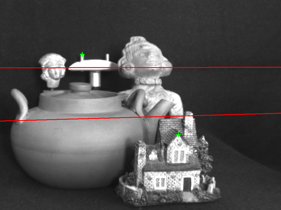
Given a pair of stereo images, epipolar rectification (or simply rectification) determines a transformation of each image plane such that pairs of conjugate epipolar lines become collinear and parallel to one of the image axes (usually the horizontal one).
The rectified images can be thought of as acquired by two new virtual cameras, obtained by rotating the actual cameras and possibly modifying the intrinsic parameters.
The important advantage of rectification is that computing stereo correspondences is made simpler, because search is done along the horizontal lines of the rectified images.
We assume here that the stereo pair is calibrated, i.e., the cameras’ internal parameters, mutual position and orientation are known. This assumption is not strictly necessary [16, 30, 23], but leads to a simpler technique and less distorted images.
Specifying virtual cameras.
Given the actual camera matrices Por and Po, the idea behind rectification is
to define two new virtual cameras Pnr and Pn obtained by rotating the actual
ones around their optical centers until focal planes becomes coplanar, thereby
containing the baseline (Figure 19). This ensures that epipoles are at infinity,
hence epipolar lines are parallel.
To have horizontal epipolar lines, the baseline must be parallel to the x-axis of both virtual cameras. In addition, to have a proper rectification, conjugate points must have the same vertical coordinate.
In summary: positions (i.e, optical centers) of the virtual cameras are the same as the actual cameras, whereas the orientation of both virtual cameras differs from the actual ones by suitable rotations; intrinsic parameters are the same for both cameras.
Therefore, the two resulting virtual cameras will differ only in their optical centers, and they can be thought as a single camera translated along the x-axis of its reference system.
Using Eq. (10) and Eq. (12), we can write the virtual cameras matrices as:
![~ ~
Pnl = K[R |- R Cl], Pnr = K[R |- R Cr].](tutorial204x.gif) | (133) |
In order to define them, we need to assign K,R, ,
, r
r
The optical centers C and Cr are the same as the actual cameras. The
intrinsic parameters matrix K can be chosen arbitrarily. The matrix R, which
gives the orientation of both cameras will be specified by means of its row
vectors:
 | (134) |
that are the x, y, and z-axes, respectively, of the virtual camera reference frame, expressed in world coordinates.
According to the previous comments, we take:
 r -
r - )/||
)/|| r -
r - ||
||
In point 2, k fixes the position of the y-axis in the plane orthogonal to x. In order to ensure that the virtual cameras look in the same direction as the actual ones, k is set equal to the direction of the optical axis of one of the two actual cameras.
We assumed that both virtual cameras have the same intrinsic parameters. Actually, the horizontal components of the image centre (v0) can be different, and this degree of freedom might be exploited to “center” the rectified images in the viewport by applying a suitable horizontal translation.
The rectifying transformation.
In order to rectify, say, the left image, we need to compute the transformation
mapping the image plane of Po onto the image plane of Pn.
According to the equation of the optical ray, if M projects to mo in the actual
image and to mn in the rectified image, we have:
 | (135) |
hence
 | (136) |
The transformation sought is a linear transformation of the projective plane (a
collineation) given by the 3 × 3 matrix H = P3×3,nP3×3,o-1.
Note that the scale factor  can be neglected, as the transformation H is
defined up to a scale factor (being homogeneous). The same result applies to the
right image.
can be neglected, as the transformation H is
defined up to a scale factor (being homogeneous). The same result applies to the
right image.
It is useful to think of an image as the intersection of the image plane with the cone of rays between points in 3D space and the optical centre. We are moving the image plane while leaving fixed the cone of rays.
|
 |
Reconstruction of 3D points by triangulation can be performed from the
rectified images directly, using Pnr and Pn.
More details on the rectification algorithm can be found in [10], from which this section has been adapted.
|
General books on (Geometric) Computer Vision are: [4, 51, 6, 12].
Acknowledgements The backbone of this tutorial has been adapted from [25]. Many ideas are taken from [12]. Most of the material comes from multiple sources, but some sections are based on one or two works. In particular: the section on rectification is adapted from [10]; Sec. 5.4 is based on [19].
Michela Farenzena, Spela Ivekovic, Alessandro Negrente, Sara Ceglie and Roberto Marzotto produced most of the pictures. Some of them were inspired by [54].
[1] S. Avidan and A. Shashua. Novel view synthesis in tensor space. In Proceedings of the IEEE Conference on Computer Vision and Pattern Recognition, pages 1034-1040, 1997.
[2] P. Beardsley, A. Zisserman, and D. Murray. Sequential update of projective and affine structure from motion. International Journal of Computer Vision, 23(3):235-259, 1997.
[3] B. S. Boufama. The use of homographies for view synthesis. In Proceedings of the International Conference on Pattern Recognition, pages 563-566, 2000.
[4] O. Faugeras. Three-Dimensional Computer Vision: A Geometric Viewpoint. The MIT Press, Cambridge, MA, 1993.
[5] O. Faugeras. Stratification of 3-D vision: projective, affine, and metric representations. Journal of the Optical Society of America A, 12(3):465-484, 1994.
[6] O. Faugeras and Q-T Luong. The geometry of multiple images. MIT Press, 2001.
[7] O. D. Faugeras and L. Robert. What can two images tell us about a third one? In Proceedings of the European Conference on Computer Vision, pages 485-492, Stockholm, 1994.
[8] A. Fusiello. Uncalibrated Euclidean reconstruction: A review. Image and Vision Computing, 18(6-7):555-563, May 2000.
[9] A. Fusiello, A. Benedetti, M. Farenzena, and A. Busti. Globally convergent autocalibration using interval analysis. IEEE Transactions on Pattern Analysis and Machine Intelligence, 26(12):1633-1638, December 2004.
[10] A. Fusiello, E. Trucco, and A. Verri. A compact algorithm for rectification of stereo pairs. Machine Vision and Applications, 12(1):16-22, 2000.
[11] R. Hartley, E. Hayman, L. de Agapito, and I. Reid. Camera calibration and the search for infinity. In Proceedings of the IEEE International Conference on Computer Vision, 1999.
[12] R. Hartley and A. Zisserman. Multiple view geometry in computer vision. Cambridge University Press, 2nd edition, 2003.
[13] R. I. Hartley. Estimation of relative camera position for uncalibrated cameras. In Proceedings of the European Conference on Computer Vision, pages 579-587, Santa Margherita L., 1992.
[14] R. I. Hartley. In defence of the 8-point algorithm. In Proceedings of the IEEE International Conference on Computer Vision, 1995.
[15] R. I. Hartley and P. Sturm. Triangulation. Computer Vision and Image Understanding, 68(2):146-157, November 1997.
[16] R.I. Hartley. Theory and practice of projective rectification. International Journal of Computer Vision, 35(2):1-16, November 1999.
[17] A. Heyden. Projective structure and motion from image sequences using subspace methods. In Scandinavian Conference on Image Analysis, 1997.
[18] A. Heyden. A common framework for multiple-view tensors. In Proceedings of the European Conference on Computer Vision, Freiburg, Germany,, 1998.
[19] A. Heyden. Tutorial on multiple view geometry. In conjunction with ICPR00, September 2000.
[20] A. Heyden and K. Åström. Euclidean reconstruction from constant intrinsic parameters. In Proceedings of the International Conference on Pattern Recognition, pages 339-343, Vienna, 1996.
[21] A. Heyden and K. Åström. Minimal conditions on intrinsic parameters for Euclidean reconstruction. In Proceedings of the Asian Conference on Computer Vision, Hong Kong, 1998.
[22] T.S. Huang and O.D. Faugeras. Some properties of the E matrix in two-view motion estimation. IEEE Transactions on Pattern Analysis and Machine Intelligence, 11(12):1310-1312, December 1989.
[23] F. Isgro and E. Trucco. Projective rectification without epipolar geometry. In Proceedings of the IEEE Conference on Computer Vision and Pattern Recognition, pages I:94-99, Fort Collins, CO, June 23-25 1999.
[24] F. Isgrò, E. Trucco, P. Kauff, and O. Schreer. 3-D image processing in the future of immersive media. IEEE Transactions on Circuits and Systems for Video Technology, 14(3):288-303, 2004.
[25] S. Ivekovic, A. Fusiello, and E. Trucco. Fundamentals of multiple view geometry. In O. Schreer, P. Kauff, and T. Sikora, editors, 3D Videocommunication. Algorithms, concepts and real-time systems in human centered communication, chapter 6. John Wiley & Sons, 2005. ISBN: 0-470-02271-X.
[26] K. Kanatani. Geometric Computation for Machine Vision. Oxford University Press, 1993.
[27] S. Laveau and O. Faugeras. 3-D scene representation as a collection of images and foundamental matrices. Technical Report 2205, INRIA, Institut National de Recherche en Informatique et an Automatique, February 1994.
[28] Jed Lengyel. The convergence of graphics and vision. IEEE Computer, 31(7):46-53, July 1998.
[29] D. Liebowitz and A. Zisserman. Metric rectification for perspective images of planes. In Proceedings of the IEEE Conference on Computer Vision and Pattern Recognition, pages 482-488, 1998.
[30] C. Loop and Z. Zhang. Computing rectifying homographies for stero vision. In Proceedings of the IEEE Conference on Computer Vision and Pattern Recognition, pages I:125-131, Fort Collins, CO, June 23-25 1999.
[31] Q.-T. Luong and T. Viéville. Canonical representations for the geometries of multiple projective views. Computer Vision and Image Understanding, 64(2):193-229, 1996.
[32] Yi Ma, Stefano Soatto, Jana Kosecka, and Shankar S. Sastry. An Invitation to 3-D Vision. Springer, November 2003.
[33] J. R. Magnus and H. Neudecker. ”Matrix Differential Calculus with Applications in Statistics and Econometrics”. John Wiley & Sons, revised edition, 1999.
[34] S. Mahamud, M. Hebert, Y. Omori, and J. Ponce. Provably-convergent iterative methods for projective structure from motion. In Proceedings of the IEEE Conference on Computer Vision and Pattern Recognition, pages I:1018-1025, 2001.
[35] S. J. Maybank and O. Faugeras. A theory of self-calibration of a moving camera. International Journal of Computer Vision, 8(2):123-151, 1992.
[36] P. R. S. Mendonça. Multiview Geometry: Profiles and Self-Calibration. PhD thesis, University of Cambridge, Cambridge, UK, May 2001.
[37] P.R.S. Mendonça and R. Cipolla. A simple techinique for self-calibration. In Proceedings of the IEEE Conference on Computer Vision and Pattern Recognition, pages I:500-505, 1999.
[38] Thomas Minka. Old and new matrix algebra useful for statistics. MIT Media Lab note.
[39] Theo Moons. A guided tour through multiview relations. In SMILE, pages 304-346, 1998.
[40] M. Pollefeys, R. Koch, and L. Van Gool. Self-calibration and metric reconstruction in spite of varying and unknown internal camera parameters. In Proceedings of the IEEE International Conference on Computer Vision, pages 90-95, Bombay, 1998.
[41] L. Robert, C. Zeller, O. Faugeras, and M. Hébert. Applications of non-metric vision to some visually-guided robotics tasks. In Y. Aloimonos, editor, Visual Navigation: From Biological Systems to Unmanned Ground Vehicles, chapter 5, pages 89-134. Lawrence Erlbaum Associates, 1997.
[42] A. Shashua. Trilinear tensor: The fundamental construct of multiple-view geometry and its applications. In International Workshop on Algebraic Frames For The Perception Action Cycle (AFPAC), Kiel Germany, Sep. 8-9 1997.
[43] A. Shashua and N. Navab. Relative affine structure: Canonical model for 3D from 2D geometry and applications. IEEE Transactions on Pattern Analysis and Machine Intelligence, 18(9):873-883, September 1996.
[44] C. V. Stewart. Robust parameter estimaton in computer vision. SIAM Review, 41(3):513-537, 1999.
[45] P. Sturm and B. Triggs. A factorization based algorithm for multi-image projective structure and motion. In Proceedings of the European Conference on Computer Vision, pages 709-720, Cambridge, UK, 1996.
[46] R. Szeliski. Video mosaics for virtual environments. IEEE Computer Graphics and Applications, 16(2):22-30, March 1996.
[47] C. Tomasi and T. Kanade. Shape and motion from image streams under orthography - a factorization method. International Journal of Computer Vision, 9(2):137-154, November 1992.
[48] Philip H. S. Torr and Andrew Zisserman. Robust computation and parametrization of multiple view relations. In ICCV, pages 727-732, 1998.
[49] B. Triggs. Autocalibration and the absolute quadric. In Proceedings of the IEEE Conference on Computer Vision and Pattern Recognition, pages 609-614, Puerto Rico, 1997.
[50] Bill Triggs, Philip F. McLauchlan, Richard I. Hartley, and Andrew W. Fitzgibbon. Bundle adjustment - a modern synthesis. In Proceedings of the International Workshop on Vision Algorithms, pages 298-372. Springer-Verlag, 2000.
[51] E. Trucco and A. Verri. Introductory Techniques for 3-D Computer Vision. Prentice-Hall, 1998.
[52] Cha Zhang and Tsuhan Chen. A survey on image-based rendering - representation, sampling and compression. Technical Report AMP 03-03, Electrical and Computer Engineering - Carnegie Mellon University, Pittsburgh, PA 15213, June 2003.
[53] Z. Zhang. Determining the epipolar geometry and its uncertainty: A review. International Journal of Computer Vision, 27(2):161-195, March/April 1998.
[54] A. Zisserman. Single view and two-view geometry. Handout, EPSRC Summer School on Computer Vision, 1998. available from http://www.dai.ed.ac.uk/CVonline/LOCAL_COPIES/EPSRC_SSAZ/epsrc_ssaz.html.