Some examples
Notes:
1. Shift-reload if any image is missing.
2. Compressed
(tar.gz) source code and images. See
readme
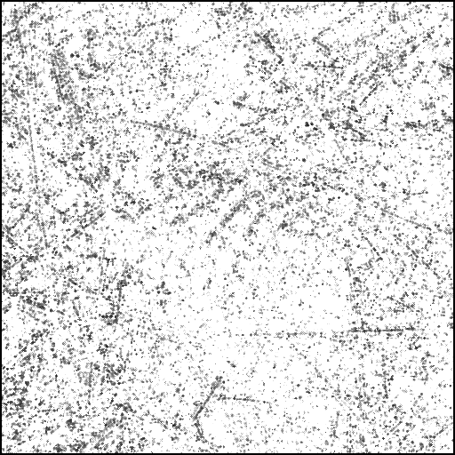
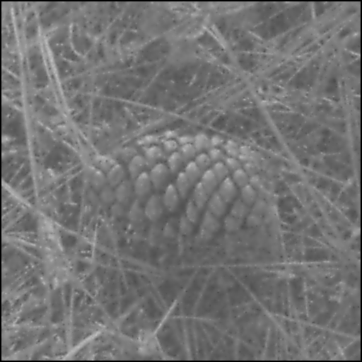
Figure 1: Example of adaptive Gaussian filtering. (a) A
pine cone image corrupted with Gaussian noise,  .
(b) Local scale map. (c) The output of 50 iterations of anisotropic diffusion,
k=10.
(d) The output of 80 iterations of anisotropic diffusion with
k=10.
(e) A chain of
  -filters,
see text for parameters. (f) The adaptive Gaussian filter.
|
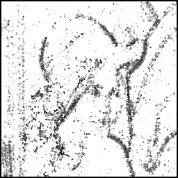
Figure 2: Example of adaptive Gaussian filtering. (a) Lenna
corrupted with Gaussian noise,  .
(b) Local scale map. (c) The output of 60 iterations of anisotropic diffusion
with k=10. (d) The output of 80 iterations of anisotropic diffusion
with k=10. (e) A chain of
  -filters,
see text for parameters. (f) The adaptive Gaussian filter.
|
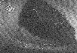
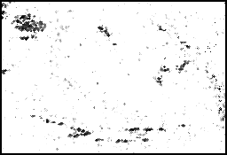
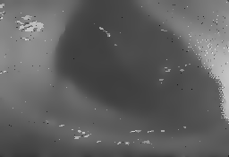
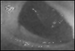
Figure 3: Example of adaptive Gaussian filtering. (a) A
human colon image corrupted with Gaussian noise,  .
(b) Local scale map. (c) The output of 100 iterations of anisotropic diffusion
with k=10. (d) The output of 120 iterations of anisotropic diffusion
with k=10. (e) A chain of
  -filters,
see text for parameters. (f) The adaptive Gaussian filter.
|
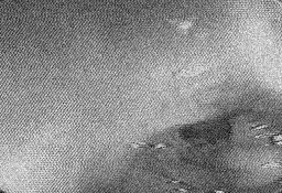
Figure 4: Example of adaptive Gaussian filtering. (a) A
human colon image corrupted with Gaussian noise,  .
(b) Local scale map. (c) The output of 100 iterations of anisotropic diffusion
with k=10. (d) The output of 120 iterations of anisotropic diffusion
with k=10. (e) A chain of
  -filters,
see text for parameters. (f) The adaptive Gaussian filter.
|

