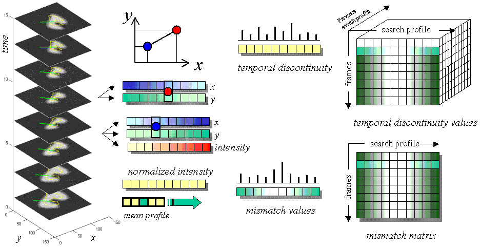
Figure 1. Obtaining the the intensity mismatch and temporal discontinuity
matrices to be used in finding a proposed ST-shape.
"Active Shape Models (ASM) are statistical models of the shapes of objects which iteratively deform to fit to an example of the object in a new image. The shapes are constrained by a Statistical Shape Model to vary only in ways seen in a training set of labeled examples." [CVOnline - ASM]
To extend 2D ASM to include temporal shape variations, we need to (1) build a statistical model of spatio-temporal (ST) shapes (time varying shapes) and (2) utilize this prior statistical knowledge along with image sequence data to segment an ST-shape.
Spatio-temporal statistics are particularly useful when dealing with a class of time-varying objects that undergoes a typical motion pattern, as in cardiography, optical signature motion recognition, or lip-reading for human computer interaction, for example.
As in 2D ASM, a single static shape is represented by a set of labels or landmarks {(xi,yi)} (x and y are the landmark coordinates, i is the landmark number). However for a time varying shape the landmark positions change with time hence the ST-shape is represented by {xi(t),yi(t)} (t denotes time).
To build a statistical model of ST-shape variations, example image sequences containing the desired object undergoing a specific motion pattern (e.g. a set of echocardiographic sequences) are collected and labeled. This yields a training set of ST-shapes. Principal Component Analysis (PCA) is then performed on the observed data; the number of observations is equal to the number of labeled image sequences (number of training ST-shapes). The number of variables in each observation is equal to: the number of frames per sequence x the number of landmarks per frame x 2 (x and y coordinates per landmark). PCA basically gives: ST_shape = mean ST_shape + weighted variation modes, in addition to the variance explained by each mode. It is important to note the ST-shapes need to be aligned prior to PCA so as not to model pose variations as shape variations.
As in the original 2D ASM formulation, a model of the image appearance around each landmark is also used (and possibly a model of how this appearance changes with time). For example by examining the image intensity profiles along a line segment passing through each landmark and perpendicular to the boundary created by the neighboring ones.
To segment a similar time-varying object in a new image sequence, we
start with an initial ST-shape model (e.g. the mean ST-shape) and an initial
pose estimate. We then
(1) find a new proposed ST-shape, (2) limit the proposed ST-shape to
agree with prior knowledge, and (3) repeat until convergence.
To find the proposed ST-shape we take into account not only image data
(match with trained appearance profiles) but also temporal continuity (Figure
1).

Figure 1. Obtaining the the intensity mismatch and temporal discontinuity
matrices to be used in finding a proposed ST-shape.
By searching along the sampled normal profiles of the all model landmarks
(at multiple image frames), each landmark can move into any of several
locations in its frame. The corresponding landmarks in the other frames
(same i but different t) can do the same. What we need is
to find is the optimal combination of new locations for all these landmarks
(specific
i, all t's) that will not only give a good
match with the prior appearance knowledge but also maintain temporal continuity.
We treat this problem as a multi-stage decision process (Figure 2).
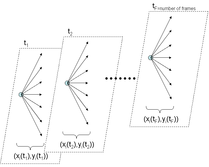
Figure 2. The different choices of the new positions of landmark
i
in all frames.
We utilize dynamic programming to solve this multi-stage decision problem,
i.e. to find the optimal path that minimizes a weighted sum of intensity
mismatch and temporal discontinuity (Figure 3).
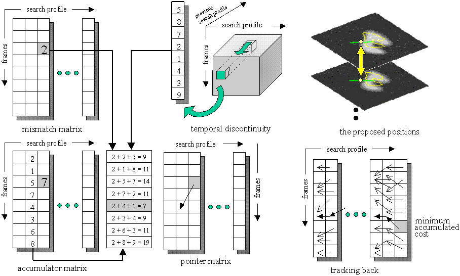
Figure 3. Utilizing dynamic programming for finding the best proposed
deformations of the ST-shape.
The result of finding the optimal path (choice of where each landmark moves to) using dynamic programming gives a proposed ST-shape. The proposed ST-shape is then limited according to the statistical model by projecting it onto an allowable spatio-temporal shape space derived from the main modes of statistical variation (Figure 4). The process is re-iterated until convergence.
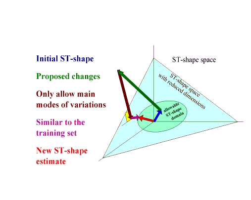
Figure 4. Constraining the deformations to an allowable spatio-temporal
shape space.
Figure 5 shows some simple examples of segmenting time-varying synthetic objects.
 ...
... ...
...
Figure 5. Segmenting time-varying synthetic objects in an image sequence
contaminated by global Gaussian noise and
(left) a missing image frame
(middle) overlapping occlusion
(right) additional localized noise
G. Hamarneh and T. Gustavsson. Deformable Spatio-Temporal Shape Models: Extending ASM to 2D+Time. British Machine Vision Conference, BMVC 2001, Vol. 1, pp. 13-22, Manchester, UK, September 10-13, 2001.
G. Hamarneh. Deformable Spatio-Temporal Shape Modeling. Licentiate Thesis,
Department of Signals and Systems, School of Electrical and Computer Engineering,
Chalmers University of Technology, 1999. Technical report 311L.