Rotational Symmetries
a Quick Tutorial

Björn Johansson

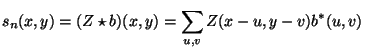
This tutorial is generated as a set of HTML pages. If you want to print the tutorial, please use the PDF version.

INTRODUCTION

The theory for operators describing rotational symmetries in image regions using orientation information was developed around 1981 by Granlund and Knutsson. It was however first mentioned in a patent from 1986, see [18,17,19]. An early related work is also [14]. For a more thorough description, see e.g. [15,6,4,12]. See also [5,3,22,2,1,21].

The theory describes modelling and detection of complex curvature, e.g. corners, circular, and star-shaped patterns. The description is based on a local orientation description in double angle representation.

The symmetries can be described in a manner invariant to color, and whether the patterns consist of edges or lines. These symmetries can serve as points-of-interest features for various computer vision tasks. Applications involve object recognition [15], recognition of object view [10], finding the non-visible center of the annual rings of a tree [20], generation of potential fields indicating possible locations for objects [21], and detection of landmarks in aerial images for use in navigation [13].

The rotational symmetries are related to the Generalized Hough Transform, GHT, which uses edges and their orientation to detect curvature, e.g. circles (see [8]). The difference is that in the GHT only positive votes give a contribution, while in the complex valued correlation used to detect rotational symmetries we will also get negative votes (see [6]). The rotational symmetries can also be more efficiently computed than the GHT.

LOCAL ORIENTATION IN DOUBLE ANGLE REPRESENTATION

The double angle representation of local orientation, $Z$, is defined as a vector, or complex number, with a phase that is double the local orientation, see [11]. Figure 1 illustrates the idea.

Figure 1: Illustration of the double angle representation.

The computer vision literature describes a number of methods to detect edges, lines, and local orientation. A convenient way to compute edges in the double angle representation is to use the image gradient:

$$Z = \vert \nabla I \vert^\gamma \ e^{i 2 \angle \nabla I}$$ (1)

where $\angle \nabla I$ means the vector angle and $\gamma$ controls the energy sensitivity.

By using the double angle representation we avoid ambiguities in the representation of boundaries between vector fields, e.g. regions in color images. It does not matter if we choose to say that the orientation has the direction $\theta$ or, equivalently, $\theta + \pi$. In the double angle representation both choices get the same descriptor $e^{i 2 \theta}$. Also, averaging the double angle description field makes sense. One can argue that two orthogonal orientations should have maximally different representations, e.g. vectors that point in opposite directions.

ROTATIONAL SYMMETRIES

There are many classes of patterns and symmetries that can be described using the local orientation in double angle representation. One class of symmetries, called the rotational symmetries, is defined as follows:

Definition: Let $r,\varphi$ denote polar coordinates. A signal $I(r,\varphi)$ is called a rotational symmetry if $\hat{Z} = Z/\vert Z\vert$ only depends on $\varphi$, where $Z$ is the local orientation description in double angle representation of the signal $I$.

Special cases are the $n$:th order symmetries:

$$Z = \vert Z\vert e^{i (n \varphi + \alpha)}$$ (2)

Note for example that the circle pattern in figure 1 has the description $Z = e^{i 2 \varphi}$. Each $n$ represents a class of patterns and $\alpha$ represents class members. Figure 2 shows some examples of gray-level patterns having the double angle description $Z = e^{i n \varphi + \alpha}$ (we ignore the magnitude $\vert Z\vert$ for a moment). The derivation of these patterns can be found in [15].

Figure 2: Examples of $n$:th order rotational symmetries, $Z = e^{i (n \varphi + \alpha )}$

The most useful classes are the 0:th order (linear symmetries), $1$:st order (parabolic symmetries), and $2$:nd order (circular, spiral and star shaped symmetries). Figure 3 shows some additional examples of gray-level patterns from these three classes when the magnitude $\vert Z\vert$ varies.

Figure 3: Examples of 0:th, 1:st, and 2:nd order rotational symmetries $Z = \vert Z\vert e^{i (n \varphi + \alpha )}$.

	$n=0$
$\alpha = 0$
$\alpha = \pi/4$
$\alpha = \pi/2$
$\alpha = 3 \pi/4$
	$n=1$
$\alpha = 0$
$\alpha = \pi/4$
$\alpha = \pi/2$
$\alpha = 3 \pi/4$
	$n=2$
$\alpha = 0$
$\alpha = \pi/4$
$\alpha = \pi/2$
$\alpha = 3 \pi/4$

Using the parameters $(n,\alpha)$ we can distinguish the patterns in different rows, but not within the rows.

Many other useful patterns can be described as linear combinations of the $n$:th order symmetries (c.f. polar Fourier transform):

$$Z = \sum_n s_n e^{i n \varphi}$$ (3)

Some examples can be found in figure 4.

Figure: Examples of gray-level patterns having a local orientation description $Z = \sum_n s_n e^{i n \varphi}$. Green= $\textrm {Real}(s_n)$, Red= $\textrm {Imag}(s_n)$, Black=$\vert s_n\vert$

DETECTION OF ROTATIONAL SYMMETRIES

The rotational symmetries are detected in a hierarchical manner. Figure 5 illustrates the idea on a simple binary test image. Note the color representation of the complex valued images. Also note that the double angle representation is non-linear, which means that the algorithm is not equivalent to linear filtering directly on the image.

Figure 5: An overview of the rotational symmetry detection algorithm.

Color representation of complex numbers

	Image, $I$
	$\downarrow$
	$\downarrow$
	$Z$
	$\downarrow$
	$\downarrow$
	$\downarrow$
$s_0$	$s_1$	$s_2$
	$\searrow$ $\downarrow$ $\swarrow$
	$\swarrow$ $\downarrow$ $\searrow$
$\check{s}_0$	$\check{s}_1$	$\check{s}_2$

First, the local orientation is computed and represented by the double angle, e.g. by using equation 1. Second, the symmetries are detected from the local orientation. One way to detect the $n$:th order symmetry is to simply correlate the orientation image $Z$ with the filter $b = g(r) e^{i n \varphi}$, i.e. 

$$s_n(x,y) = (Z \star b)(x,y) = \sum_{u,v} Z(x-u,y-v) b^*(u,v)$$ (4)

where $^*$ means complex conjugate and $g(r)$ is some suitably chosen window function, for example a Gaussian function. A high magnitude $\vert s_n\vert$ indicate a high probability that the pattern belongs to class $n$. The argument $\angle s_n$ corresponds to the class member (c.f. $\alpha$ in equation 2).

Another, more efficient, way to compute the symmetries is to use the parameters from a local polynomial expansion model of $Z$. A second degree polynomial is sufficient to detect symmetries of order $\vert n\vert \leq 2$:

$$Z(x,y) \sim r_1 + r_2 x + r_3 y + r_4 x^2 + r_5 y^2 + r_6 xy$$ (5)

The polynomial expansion is computed in each local area using weighted least squares. The weight is a Gaussian function with std $\sigma$, which controls the size of the local window. The expansion can be efficiently computed in one or several scales by means of convolution with a small set of 1D filters, see [15], [9], [7].

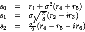
From the parameters ${\bf r} = (r_1, ..., r_6)$ we compute the symmetry responses $s_0$, $s_1$, $s_2$ as

$$\begin{array}{ccl} s_0 & = & r_1 + \sigma^2 (r_4 + r_5)\\ s_1... ...\\ s_2 & = & \frac{\sigma^2}{2} (r_4 - r_5 - i r_6) \end{array}$$ (6)

Sometimes it may be desirable to classify the response into one symmetry order $n$, for example if we want to use $s_1$ as a detector for curvature and corners, and $s_2$ as a detector for circle and star shapes. As can be seen in figure 3, the first order symmetries also approximately include linear symmetries. The same overlap holds between other symmetries (corners give for example a fairly high magnitude $s_2$, because they are approximately ``half circles'' etc.). Hence, to further make the responses more selective we can apply an inhibition scheme. The basic idea is that if one magnitude is high, the other ones should get low. See [15] and [16] for suggestions on how to implement this.