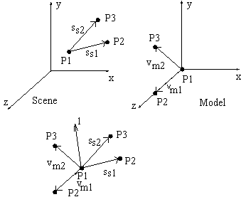
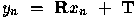
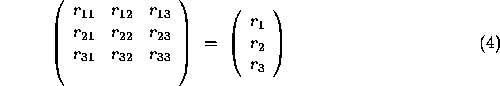
Figure 2, below, illustrates the basic problem. There are two matching point sets or, alternatively, a matching point and two vectors in the model which match two vectors in the scene . There are several different transformations which superimpose the model set on the scene set (or vice versa).

Figure 2: Transformation of 3 points, or a point-vector-vector

These can be combined to form

representing the point to be transformed as in homogeneous coordinates. If is a rotation matrix in 3D orthogonal space, then and the determinant of is 1. Representing and so on this gives 6 constraint equations,

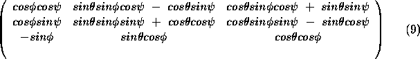
The first intuitive approach to define a rotation matrix might be the fixed axis method , e.g.

• Translate point to the origin
• Rotate by about the original x-axis (positive rotation is from y to z)
• Rotate by about the original y-axis (positive rotation is from z to x)
• Rotate by about the original z-axis (positive rotation is from x to y)

This leads to a rotation matrix formed by the concatenation of the matrices for the three single angle rotations about the fixed axes,

Note also that the angles can be recovered, , and .

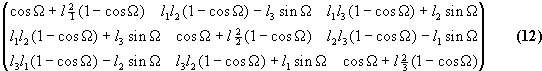
A second method to define a rotation matrix, illustrated in Figure 2, above, is based on a rotation about an arbitrary axis, , by an angle . ,

and is defined

The rotation matrix is

Re-arranging, we can also express and in terms of the rotation matrix elements.

The trace of a square matrix is defined as the sum of the diagonal elements, . N is a normalisation operator, .

[ Pose Estimation: Contents | Least squares estimation of 3D pose ]

Comments to: Sarah Price at ICBL.