 .
In most cases, this distribution can be approximated by a
normal probability distribution function,
.
In most cases, this distribution can be approximated by a
normal probability distribution function,  ,
of standard deviation,
,
of standard deviation,  ,
where x is the value of intensity, depth or other function.
,
where x is the value of intensity, depth or other function.


In sensing image brightness, or indeed depth, it is inevitable that the
individual picture element (pixel) values will be subject to the corrupting
effect of noise both at sensing and amplification of the resulting electronic
signal.
Thus if several measurements are taken of the same pixel intensity whilst
viewing the same scene, there will be distribution of measured value about
a mean intensity, .
In most cases, this distribution can be approximated by a
normal probability distribution function, ,
of standard deviation, ,
where x is the value of intensity, depth or other function.

where

and

The pixel intensity stored in the digital framestore or computer is further quantised, i.e. it is stored as one of a finite number of digital values, typically 256 values when stored as a single byte. The effect of quantising the original analogue signal by analogue to digital conversion introduces a further source of inaccuracy, i.e. quantising error or loosely, quantising noise. This can be expressed with regard to the original digital signal in terms of the mean squared error signal,

or the root mean square noise (cf ),

where q is the width of the region of uncertainty of the signal level. In designing a video input signal, it is desirable to equate the "noise" levels introduced by the quantisation and Gaussian noise effects. For a CCTV camera, 8-bit quantisation is certainly adequate, and in practice it is likely that only the first 6 bits are significant.
Because the computer can only store a finite number of measurements of image intensity etc., spatial sampling is also required. In effect the image on the camera "retina" is sampled according to a predefined grid, normally rectangular, which may be 512 by 512 elements to obtain TV quality for example. Each number in the sampled image then represents the average image irradiance over a small square or rectangular area. The effect of this tessellation of the image into the pixel elements will have further effects on the image data. In general, the optimum separation of the sampling pixels is related to the rate of transition of intensity of the image data by the sampling theorem, which states that

where  is the maximum frequency of intensity change in the
original image, a function of the filtering introduced both by the optical and electronic pre-processing.
If the sampling interval is too large with respect to the image function then the phenomenon of
aliasing occurs. In this case, undersampling of the high frequency components results in spurious low frequency signals being generated, interacting with the real image and producing unusual effects.
Figures 3, 4, 5, and 6, below, show the effect of
increasing the sampling frequency and number of digital signal levels.
is the maximum frequency of intensity change in the
original image, a function of the filtering introduced both by the optical and electronic pre-processing.
If the sampling interval is too large with respect to the image function then the phenomenon of
aliasing occurs. In this case, undersampling of the high frequency components results in spurious low frequency signals being generated, interacting with the real image and producing unusual effects.
Figures 3, 4, 5, and 6, below, show the effect of
increasing the sampling frequency and number of digital signal levels.
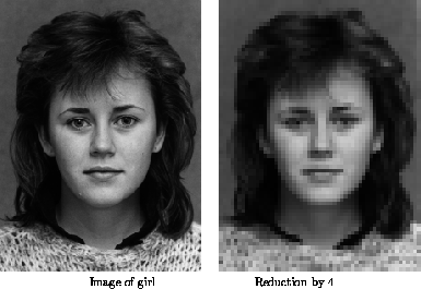
Figure 3: The effects of sampling
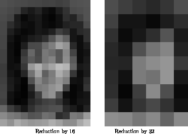
Figure 4: The effects of sampling
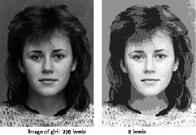
Figure 5: The effects of quantisation
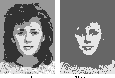
Figure 6: The effects of quantisation


[ Signals in one and two dimensions |
Convolution in two dimensions ]

Comments to: Sarah Price at ICBL.
(Last update: 4th July, 1996)