Given the binary image, it is possible to compute certain geometric properties (and in the case of multiple component images topological properties), such as object area, perimeter length etc. These properties can be used to uniquely determine the position, orientation and identity of a component in the camera field of view with respect to a known database of object models.
In practice this technique can be applied to a database of simple industrial components, to identify them by the silhouettes of their stable states. Various specialised lighting techniques may be applied to obtain a good image of this nature, including backlighting (e.g. an overhead projector), laser striping, and colour filtering (e.g. a background painted with fluorescent red paint and illuminated with UV light increases the contrast between the background and any non-fluorescent object lying on it; a red filter further enhances the contrast). In general we must define a set of geometric features which uniquely identify each object. For example, it is possible to use the following set of features which are orientation independent.
The details of these calculations are relatively straightforward and are covered in Calculation of Geometric Properties.
The set of features, f1-7 may be measured rapidly and simply from the binary image data and need to be used to classify the observed image within a given object class, however there will be variation in values due to the effects of camera translation and rotation, camera noise, quantisation noise etc. The method of classification should deal with these variations. Two approaches available are statistical classifiers and decision trees.
 of values to be compared with stored information
for each object class
of values to be compared with stored information
for each object class  .
The ``best'' match is defined by Bayes theorem
to be the one that maximises:
.
The ``best'' match is defined by Bayes theorem
to be the one that maximises:
In general, this will depend on the covariance matrix showing how features depend on each other, but if the features can be considered as identically distributed, normal and independent, then this justifies the use of the Euclidean distance to the mean of each feature vector. In most cases it is reasonable to assume that the measured distribution of a particular feature variable will be normal about the mean value. Thus the classification is performed by finding the class that minimises:
This method can be refined to use a weighted sum, or correlation applied to give a similarity weighting between classes. (Further details Schalkoff p258.) Figure 5 shows an example of a 2 class, 2 feature problem; the elliptical lines represent equal probability contours in the two dimensional feature space. If the distributions are normal, then the projections of the two dimensional functions onto the x and y axes will look like simple one-dimensional normal curves. In principle, it may be difficult to separate the two classes in either one dimensional feature space, but they may be sufficiently distinct in the two-dimensional feature space. This forms the basis of the statistical classification technique which is not considered fully here.
 and the variance is
assumed constant for all distributions.
and the variance is
assumed constant for all distributions.
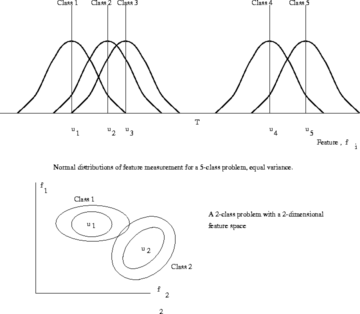
Figure 5: Single feature measurement for a five class problem
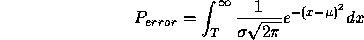
To distinguish between the feature classes, (1,2,3) and (4,5), the threshold value should be set midway between class 3 and class 4; the larger the gap, the more reliable is the classification of the object into one of the two possible sets. The probability of misclassification of object 3 as object 4 ( or vice versa ) is given by
Further decisions are required to separate objects 1 from 2 and so on. A binary decision tree is constructed in which those features which have the largest gaps are used initially and the problem is treated recursively for each of the two sub-trees. The general principle is illustrated in Figure 6
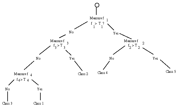
Figure 6: A decision tree for a five class problem
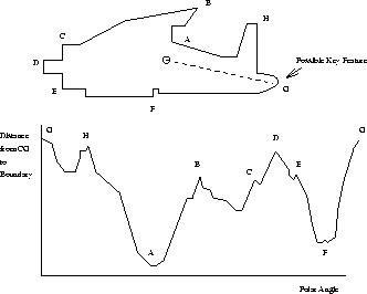
Figure 7: Determining the orientation of a classified figure
 [ Intensity Histograms |

Author:: Andrew Fitzgibbon at the Department of Artificial Intelligence, University of Edinburgh