 |
D.R. Roberts and A.D. Marshall
Department of Computer Science,
Cardiff University
PO Box 916, Cardiff. CF2 3XF, U.K.
Email: dave@cs.cf.ac.uk
Many machine vision tasks, e.g. object recognition and object inspection, cannot be performed robustly from a single image. For certain tasks (e.g. 3D object recognition and automated inspection) the availability of multiple views of an object is a requirement.
This paper presents a novel approach to selecting a minimised number of views that allow each object face to be adequately viewed according to specified constraints on viewpoints and other features. The planner is generic and can be employed for a wide range of multiple view acquisition systems, ranging from camera systems mounted on the end of a robot arm, i.e. an eye-in-hand camera setup, to a turntable and fixed stereo cameras to allow different views of an object to be obtained.
This paper outlines a viewpoint planning approach that encompasses all the above vision system types.
Considerable research in machine vision has been directed at object recognition and object inspection. For complete 3D recognition or inspection several distinct views of the object are usually required. However, until recently, little consideration has been applied towards identifying strategies for selecting such viewpoints. Usually fairly simplistic methods or assumptions (e.g. fixed angular steps) are made when selecting viewpoints. If careful a priori or on-line determination of viewpoints can be made then benefits may include improving the quality, efficiency and/or reliability of subsequent processing and object recognition tasks. In many instances object inspection and, often, object recognition will be performed in controlled environments where a CAD model of the object of interest may be available. It is worthwhile looking to exploit stored knowledge of the object and its environment to determine viewpoints that improve the performance of these tasks, e.g. reducing the amount of redundancy in data capture and the time cost of capturing this data.
This paper describes a planning system that has been developed to select viewpoints suitable for a variety of machine vision tasks, e.g. recognition and inspection. As input, the planner takes a description of the vision work-cell, a CAD boundary representation model of the object of interest, and a description of the visibility of each of the objects faces. The work-cell description defines lens optical settings and other metrics that depend on the multiple view acquisition system used, e.g. if multiple views are obtained from a fixed camera and turntable then these metrics would include camera position and orientation relative to the turntable and turntable step size. For a given object face, its visibility is defined by a generalised cone that bounds the directions along which there is an unobstructed view of the face. Additional constraints can also be specified for the purpose of adapting the planner to search for viewpoints suitable for specific applications.
Planning is performed in two stages: (1) features are grouped into sets that are suitable for viewing from a common viewpoint (viewpoint planning), and (2) viewpoints are selected to view these feature groups (viewpoint selection).
Two approaches to sensor and viewpoint planning are possible, these can be described as follows: (a) Determine the next viewpoint on the basis of information derived from the analysis of the current and previous views, or (b) Determine a suitable set of viewpoints prior to beginning the vision task.
The first approach is more applicable when there is no model of the viewed object available. Planning of this type has been used for the automatic generation of object models, acquiring images that can be used to represent a scene or an object, and for view selection for the purpose of visually searching a scene[1,2,3].
The second approach is suitable when a CAD model of the object is available. Possessing an understanding of the shape of the model allows more complex and specific plans to be generated that exploit the available knowledge. This form of sensor planning has been developed for several different purposes, for example object recognition [4,5], general robot vision tasks [6], inspection of loose tolerance objects [7], and accurate inspection [8]. Both Cowan [4] and Tarabanis [6] have developed sensor planning systems that determine suitable sensor positions for viewing a feature by applying constraints to the set of possible viewpoints. Tarbox [7] has looked at viewpoint planning to allow the complete surface of an object to be seen.
For a complete review of previous methods readers are referred to the Research report
[15] URL:http://www.cs.cf.ac.uk/Research/Rrs/1997/detail007.html
In general, the problem of selecting a set of viewpoints to allow the whole of an objects surface becomes a tradeoff between two rather contradictory aims -- trying to minimise the number of viewpoints while trying to ensure that the viewpoints selected yield views of each face as close to the best view as possible. This is particularly important for an application where accuracy is a concern, e.g. visual inspection. The best view of a feature or a group of features can be defined in several ways. In general, the best view of an object face is obtained when it is viewed head on [9]. This occurs when the viewing direction is the inverse surface normal of the face. For a curved surface this can either be approximated by the average surface normal or the surface can be approximated by planar facets that are then considered separately. However, there is no guarantee that a face may be visible from this direction corresponding to the inverse surface normal. A more robust definition of the best view is the direction that lies within the faces visibility region and has the smallest angular offset from its inverse surface normal.
A problem that may arise when the goal is to minimise the number of views is evident if three faces of a cube sharing a common vertex are considered. Two views would be capable of capturing the complete surface data. It is obvious that the best view of any of these faces cannot be obtained since it would require that the other two be at oblique glancing angles to the cameras line of sight. Therefore, for a group of faces, the best view may be defined as the direction that is simultaneously a minimum angle from each of the corresponding surface normals [9].
The system we have developed interrogates a stored CAD model of the object to be inspected to generate a suitable strategy for acquiring data from multiple views. The primary data required for inspection are range images which cover the inspection object, thus in this paper, references to `features' will imply faces. Currently the system is restricted to dealing with polyhedral objects and hence curved surfaces must first be approximated by such methods as planar faceting. While faceted models may not in general be accurate enough for geometric inspection to engineering tolerances, at this stage, we are only concerned with planning the set of range images to be captured, and for this a polyhedral approximation is sufficient.
The first stage of our planning system is concerned with configuring the workcell. The cameras and laser scanner then remain static for all sensing operations. This is for practical reasons, since it eliminates the need for continued re-focusing and re-positioning, which is complex, inefficient to automate and makes it difficult to retain accuracy. Hence it is necessary to ensure that for all sensing operations, all the relevant features lie in focus in both cameras and also lie within the field-of-view of both cameras and the laser. These are used as constraints to determine suitable values for the various parameters at the configuration stage. The variable parameters are the disparity between the stereo cameras, the distance that they lie from the inspection object, and suitable choices of lens settings.
The next stage is planning the set of viewpoints given the set-up determined in the previous phase. The number of sensing operations that is needed and the appropriate object orientations are determined by analysing the visibility of the inspection object. This involves determining the sets of directions along which faces are entirely visible. This ensures that selected sensing directions view the entire face. From this information a series of viewpoints may be chosen that allow all selected features to be inspected with a minimum number of operations. In the following, a viewpoint is taken to mean the relative orientation of the object with respect to the sensors.
The configuration of the workcell is an important factor in aiding the acquisition of suitable and accurate data. To accomplish this automatically it is necessary to identify both the fixed and variable parameters that describe the configuration of the workcell and sensors. Those parameters that are fixed must be allowed for and compromises will have to be made to accommodate these. The variable parameters can be set such that they provide the best configuration for the succeeding tasks.
Although the process of configuring a workcell has been approached with generality in mind, it has inevitably been tailored to our particular system.
Currently we are only interested in determining suitable configurations that allow the planning system to acquire high quality images. The problem of determining the optimum workcell configuration is not considered, this is an interesting problem in itself.
The primary purpose of this pre-planning stage is to ensure that for all selected imaging operations the data acquired is in focus and the corresponding features are visible to the camera. Therefore for this purpose, we are interested in the fields-of-view of the camera lenses and their depth-of-focus. Since the data needed is range data from an active stereo camera system, these camera parameters must be extended to apply in stereo.
The lenses on both cameras are controllable zoom lenses. This allows suitable combinations of aperture, focal length and focus distance to be set. Once these intrinsic lens parameters have been determined they then remain constant for the inspection of each part of the object. This eliminates the need for re-calibration of the system, which is not possible for an inspection system since relationships between features will be lost.
In our inspection system, the range of positions and orientations the cameras can take is fairly limited. This dictates the configuration somewhat, however, should we wish to relax this at any time then our configuration process is flexible enough to allow for this.
In the following sections we present our method for determining both sensor placement and the lens settings. This is done by considering the stereo field-of-view and the stereo depth-of-field. Although they are presented separately they are dependent on each other, this dependency will be discussed at the end of the section.
Once suitable camera placements and lens parameters have been found, they must be oriented such that the optical axes of the two cameras intersect at the centre of the turntable. This can be ensured during the initial calibration of the system. A suitable calibration chart is placed on the turntable, the chart is then imaged at different orientations allowing the axis of rotation and hence the centre of the turntable to be found. The distance that each camera lies from the turntable can also be estimated at this stage.
The field-of-view of a camera determines all points that are visible to the camera. It is a conical region whose apex lies at the optical centre of the lens and whose angle depends on the focal length of the lens.
For simplicity, certain assumptions have been made. The first assumption is that the field-of-view of a camera is a right circular cone. The field-of-view of a real camera is rarely symmetrical: in general it will be a flattened rectangular cone. However, by taking the field-of-view as the minimum angular dimension, it is guaranteed that only space that is actually visible to the cameras is being considered. The second assumption is that the angular field-of-view of the laser is not considerably different from that of the cameras: if the laser is either mounted on one of the cameras or placed between the two, it is a reasonable assumption that all points visible to both cameras are also within the field-of-view of the laser.
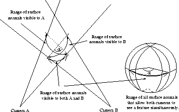
We define the stereo field-of-view as the set of all the points that are simultaneously visible to both cameras. For converging cameras, that are generally used in stereo set-ups, this is a closed region of overlap, as shown in figure 1.
A further constraint is that only features whose Gaussian image (a description of a surfaces shape found by intersecting its surface normals with the unit sphere) is wholly within the range of directions on the sphere shown in figure 2 are simultaneously visible to both sensors. This poses additional problems when curved surfaces are considered. However, this is an issue that can be dealt with by means of visibility calculations and is discussed fully in section 3. At this stage we simply wish to configure the system such that the inspection object will lie inside the region of overlap for all imaging operations, the more restricted case is not considered at this stage. It is worth noting though, that this constraint could be incorporated by requiring that only those features whose Gaussian image is within this range must lie within the region of overlap. Currently we take the following, simpler approach.
The turntable is marked with concentric circles of known and varying radii. Placing the object on the turntable allows us to choose a circle of sufficient radius to contain the object. This radius is then taken as that of the bounding sphere of the object. By removing the need to reason with complex convex shapes (since we would require that the convex hull of the object is visible) we can deal with the simpler geometry of the sphere. This operation forms part of the initial calibration of the system.
Now the problem has been reduced to finding the best configuration such that the sphere lies within the common region of view, i.e. such that the object will appear as large as possible in both images. For the general case of fixed lenses of known focal lengths this is a non-trivial optimisation problem.
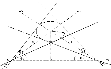
Both intrinsic and extrinsic camera parameters determine this region. The distances that the cameras lie from the turntable and the focal length of the lens determine how large the object appears in the image for the fixed lens case. The baseline size determines the range of surface normals that are commonly visible and the camera orientations determine the size of the area of overlap.
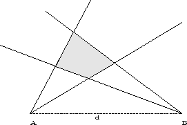
The radius (r) of the sphere (figure 3) inside which the inspection object
is contained is known. The space that lies within the overlap of the cameras
fields-of-view is dependent on the focal length of the lenses (f1, f2), the angles
(![]() ) which the optical axes of the two cameras make with the baseline,
and the disparity (d) between the cameras. A compromise must be made between the
following requirements: making the object as large as possible in each view, ensuring a
reasonable amount of overlap between the two views, and a sufficiently large disparity to
ensure accurate depth values.
) which the optical axes of the two cameras make with the baseline,
and the disparity (d) between the cameras. A compromise must be made between the
following requirements: making the object as large as possible in each view, ensuring a
reasonable amount of overlap between the two views, and a sufficiently large disparity to
ensure accurate depth values.
For each lens we choose a suitable focal length such that the bounding sphere of the object fills the field-of-view of both cameras. This is feasible since the field-of-view varies smoothly with the focal length settings. The difference in the distance that the turntable lies from each lens is not going to be significant and so the difference in the size of the features in corresponding stereo images will be small. Suitable focal lengths can be found from:
fi = targetsize/( 2 tan ( invsin(r* sin(phii)/h)) for i = 1,2
The angle that the optical axes make with the baseline ![]() and
and ![]() is
related to the baseline size and the perpendicular distance to the turntable. The smaller
the disparity the larger the range of feature orientations that will be visible to both
cameras, this was shown in figure 2. However this is just stating the
stereo correspondence problem, trading off making the disparity large to allow accurate
depth readings against making the disparity small to ensure a greater overlap of features
in the resulting images.
is
related to the baseline size and the perpendicular distance to the turntable. The smaller
the disparity the larger the range of feature orientations that will be visible to both
cameras, this was shown in figure 2. However this is just stating the
stereo correspondence problem, trading off making the disparity large to allow accurate
depth readings against making the disparity small to ensure a greater overlap of features
in the resulting images.
For any given lens, only points that lie at a single particular distance will be perfectly in focus, and points lying within a range of distances about this value will be blurred by an area that is smaller than the minimum dimension of a camera pixel. The size of this range determines the cameras depth-of-focus.
Using a zoom lens allows the focal length and aperture to be changed and hence allows a suitable depth-of-focus to be chosen. Given the radius of the sphere placed around the object, the closest points will lie within a distance equal to the difference of the distance between the optical centres of the camera and turntable centre and the radius of the sphere. The farthest point will be equal to the sum of these two lengths.
We know the resolution of the imaging system, the focal length and the desired depth-of-focus, i.e the difference between the minimum (Dmin) and maximum distances (Dmax) at which points must be in focus. By solving the following pair of equations, suitable combinations of aperture setting and focus distance can be found to ensure the required depth-of-focus (Krotkov, 1989).
D = f Dmax(a + c) / ( af + c Dmax),
D = f Dmin(a + c) / ( af - c Dmin)
Where D is the focus distance, f is the focal length of the lens, a is the aperture diameter and c is the circle of confusion diameter.
In our stereo system, this must be done for both cameras. This is to ensure that the features being inspected are focused in both cameras at the same time.
By treating the above two lens properties separately there is a certain amount of conflict. This is because both depend on the value of the focal length of the lenses. Lenses of suitable focal lengths are chosen to try and maximise the size of selected features in the image plane, the problem is then attaining the required depth-of-field. The depth-of-field is dependent on the lens aperture diameter, the focus distance and the focal length. The only variable here is the aperture setting, values for the other two have been determined. This is enough to allow us to ensure that all features are in focus, however the problem of suitable lighting is now important. When the aperture diameter is reduced so is the amount of light that enters the camera, therefore to resolve this there is a need to increase the intensity of artificial lighting. This is undesirable since it suggests the need to consider planning the workcell lighting as well. The problem of light is not so important for our specific needs since the images that we obtain are laser spots. If the images acquired were grey-scale or colour images of the inspection object then important detail could be lost under poor lighting conditions.
There is a certain degree of scope for avoiding aperture diameters that are very small
when using a zoom lens. The purpose of examining the cameras field-of-view was to ensure
that all features are wholly visible and also to try and make features as large as
possible in the resulting images. Having completed this stage, if the focal lengths are
shortened the simple result is that the field-of-view becomes larger and the features
become smaller in the corresponding images. Therefore, it is also possible to adjust the
focal lengths to help obtain the necessary depth-of-field.
In this section, a description is given of the methods that have been used to develop our viewpoint planning strategy.
The viewpoint planning problem can be conveniently defined as a search problem of a type that has been comprehensively described in artificial intelligence literature [10]. Taking this approach, a search space needs to be defined in which potential solutions can be evaluated in an attempt to find the best solution.
It may be intuitive to define the search space in terms of what is being sought, i.e. viewpoints. Such a representation is called an aspect graph [11]. Nodes in this graph correspond to a set of viewpoints from which the same topological entities are visible, and arcs correspond to transitions from one aspect to another caused by movement in viewpoint that results in a change in the visible topology of a viewed object or scene. There are, however, drawbacks in this representation, the most relevant of these are the complexity in generating aspect graphs and the potentially huge search spaces (even for moderately simple objects) that may result [12]. Another disadvantage of this representation is that the aspect graph deals with the visibility of object features and, hence, further constraints that may affect viewpoint selection are not easily incorporated into the representation.
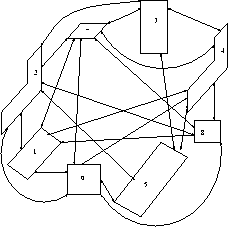
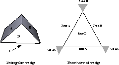
For these reasons an alternative representation has been investigated. Rather than deal with viewpoints, a set of faces suitable for viewing from a common viewpoint are sought. In our representation the search space is defined by a graph in which the nodes correspond to faces of the object of interest and arcs between two nodes represent both faces satisfying all necessary constraints simultaneously. Hence, if face visibility is the only constraint being used then an arc would connect two nodes if the two corresponding faces are visible from a common point (or region) in space. This representation has the advantage that it can be generated from geometric information readily held in the stored CAD model and visibility information computed at an earlier stage[13] (other relevant information relating to other constraints on a viewpoint may also be incorporated). The graph also has definite manageable size, n nodes for n faces, and knowing the exact size of the graph before construction leads to a simpler representation of the structure. The graph representation of a simple object using visibility as the only constraint on viewpoint is shown in Fig. 4.
The graph can be conveniently and efficiently represented as a 2 dimensional array. Elements of the array have values determined by the constraints imposed on pairs of faces. For example, the graph in Fig. 4 using visibility constraints and surface normal information would be stored as the array shown in Table 1.
| C1 | C2 | C3 | C4 | C5 | C6 | C7 | C8 | |
| R1 | - | 90 | - | 90 | - | 90 | 90 | |
| R2 | 90 | - | 90 | - | 90 | 90 | 90 | 90 |
| R3 | - | 90 | - | 90 | 90 | - | 90 | - |
| R4 | 90 | - | 90 | - | 90 | 90 | 90 | 90 |
| R5 | - | 90 | 90 | 90 | - | 90 | - | - |
| R6 | 90 | 90 | - | 90 | 90 | - | 90 | |
| R7 | 90 | 90 | 90 | - | 90 | - | 90 | |
| R8 | 90 | 90 | - | 90 | - | 90 | - |
In the array shown in Table 1, entries in the range ![]() correspond to the angle
correspond to the angle ![]() between the surface normals of two compatible faces.
Hence, entries in this range correspond to two faces that satisfy all necessary
constraints simultaneously and consequently to two connected nodes in the graph. Incompatible faces,
i.e. those that do not satisfy all constraints simultaneously and hence relate to
unconnected nodes in the graph are represented by entries with a null (-) value.
When other constraints are imposed for which there are values that also have properties
that are suitable to distinguish faces suitable for viewing from a given viewpoint, these
can be combined with the surface normal values and any other meaningful values into a cost
function. The cost function is then used as a basis for determining faces to be viewed
from a particular viewpoint. The main aim here is to highlight that a flexible, generic cost
function has been developed -- space limitations prevent further discussion and illustration of this
matter here, for further results refer to [14].
between the surface normals of two compatible faces.
Hence, entries in this range correspond to two faces that satisfy all necessary
constraints simultaneously and consequently to two connected nodes in the graph. Incompatible faces,
i.e. those that do not satisfy all constraints simultaneously and hence relate to
unconnected nodes in the graph are represented by entries with a null (-) value.
When other constraints are imposed for which there are values that also have properties
that are suitable to distinguish faces suitable for viewing from a given viewpoint, these
can be combined with the surface normal values and any other meaningful values into a cost
function. The cost function is then used as a basis for determining faces to be viewed
from a particular viewpoint. The main aim here is to highlight that a flexible, generic cost
function has been developed -- space limitations prevent further discussion and illustration of this
matter here, for further results refer to [14].
Given the representation that has been chosen, the first stage of the planning problem can be stated as trying to group faces together into sets that can be viewed from a common viewpoint in such a way that a minimum number of viewpoints is required to view all faces. Described in this way, the problem is essentially one of set partitioning. If a minimum number of views is desired then these partitions are disjoint subsets. This is ignoring the possibility that disjoint sets might not be desirable for object inspection where feature inter-relationships may be needed. However, if the views are registered sufficiently well the relationships may be determined anyway. A solution to finding the minimum number of viewpoints is to generate all possible partitions and by applying some heuristic to each, determine which forms the best plan. Looking at all combinations, i.e. all viewpoint plans, would guarantee the minimum solution is found. For simple objects, analysing all possible combinations is possible. However, for objects with even a moderate number of faces, the complexity increases dramatically[16].
A better approach is to consider all possibilities by searching the graph in a breadth first fashion. However, the computation time to perform a complete search is not tractable. Therefore, rather than attempt to find the best possible plan it is more logical to look for an acceptable plan that can be computed in a reasonable time. Our planning method computes an approximation to the best viewpoint plan. First, the largest set of faces suitable for imaging from a single common viewpoint is sought. These faces are then removed from the set of all faces and the largest set of suitable faces is found from the remaining faces. This procedure is continued until all faces have been considered. In the graph representation used, two faces are suitable for viewing from a common viewpoint if their corresponding nodes are linked by an arc. For a set of n faces to be suitable for viewing from a common viewpoint, the node corresponding to each face in the graph must be connected to all n-1 other nodes corresponding to the other n-1 faces. Therefore, the search is for the largest fully connected subgraphs, or cliques. Determining the maximum clique of a graph is an NP-hard problem.
A number of heuristics can be applied to aid solution to this problem[17]. The approach taken to our viewpoint planning problem is one of constraint satisfaction. Instead of minimising the number of views, it attempts to maximise the number of faces satisfying all constraints. Therefore, the search is for the largest set of faces simultaneously satisfying all constraints.
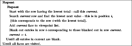
Our solution allocates object faces into groups that satisfy all constraints simultaneously. We use the concept of a clique to find a set of object faces suitable for viewing from a common viewpoint. Our algorithm (Table 2) maintains a current viewpoint list holding the tags of those faces that are simultaneously visible and have been deemed by the algorithm as suitable for imaging from a common viewpoint. Face tags are added to the current viewpoint list on the basis of which has the lowest row sum in the array representation (see, for example, Table 1). When the longest possible list has been found, (this occurs when the row in the array representation corresponding to the current face has all blank entries), the nodes in the list are removed from the graph. The faces in the list at this point correspond to a set of faces that will be viewed from a common viewpoint. The search is then repeated on the graph to find the next viewpoint, this repetition continues until all nodes have been removed from the graph. Each viewpoint list found corresponds to an approximation to the maximum clique in the current state of the graph.
The rationale behind the strategy for choosing the first (and successive) face is that blanked entries, corresponding to unconnected nodes in the graph, are given a high score. Hence, the row with the lowest total will have the least blanked entries (i.e. has common visibility with most other faces) and, depending on constraints set, also has closest surface orientation to all other faces. For these reasons, using this selection strategy is likely to choose a good first (next) node.
When visibility is a constraint on viewpoint selection, applying the algorithm as it is given may compute cliques that do not correspond to acceptable face groupings for viewing from a common viewpoint. An example of such an instance is shown in Fig. 5, where faces A, B and C do not have a common visibility region. However, in the graph corresponding to this object, {A, B, C} is a clique. To avoid occurrences of these cliques, a single intersection test on the corresponding visibility regions must be performed by the underlying geometric modeller for each node being added to a clique (face being added to a viewpoint list). This ensures that all corresponding faces have a common visibility region. This operation is a basic geometric modeller operation and introduces no significant overheads to our method as many more general intersections are being performed already.
In this section, consideration is given to the second phase of planning, selecting viewpoints to view face groups selected by the algorithm given in the previous section. Methods for viewpoint selection are given for two different view acquisition setups.
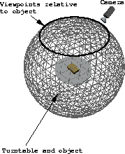
In this configuration, it is assumed that a camera is mounted on a robot arm that has sufficient dexterity to position the camera at any viewpoint relative to the object. Potential viewpoints surrounding the object define a viewsphere. The camera remains at a fixed distance to the object, determined at a preliminary calibration stage [13]. The distance between the object and camera defines the radius of the viewpshere.
Output from the planning algorithm is in the form of a list of face groups that are
suitable for viewing from a common viewpoint. To determine the region of acceptable
viewpoints for viewing all faces in a group, the visibility regions of the faces in the
list are intersected. The result is a generalised cone from which any direction inside is
capable of viewing all the corresponding faces. Intersecting this cone of view directions
with the viewsphere results in a region of viewpoints on the viewsphere that are suitable
for viewing the face group. This region of viewpoints can be considered as representing a
set of candidate viewpoints, from which the best is chosen, i.e. the viewpoint that
has a minimum angle to all corresponding face normals (or where necessary, the closest
direction to this lying inside the intersected visibility regions). The chosen viewpoint
is then returned as a point on the viewsphere.
Consideration is now given to selecting viewpoints that are suitable for viewing the face groups selected by the planner using a fixed camera and a turntable to vary the viewpoint relative to the viewed object. The turntable only has one degree of freedom, an angular rotation about its centre, hence the range of possible viewpoints is also restricted to a single degree of freedom about the object. It is assumed that the camera has been configured so that its optical axis is directed at the centre of the turntable.
In this setup, a viewsphere (Fig. 6) is defined by the turntable centre and the camera position. Essentially, the algorithm given made no assumption on possible viewpoints and so a viewpoint required to view a chosen set of faces could potentially lie at any point on the viewsphere. In this setup possible viewpoints that can be achieved are restricted to those lying on a circle on the viewpshere determined by the pose of the cameras.
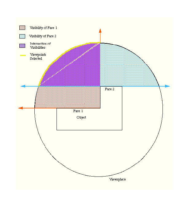
The method given previously for finding the region of acceptable viewpoints to view a group of faces (intersecting the visibility regions of the corresponding faces to find viewpoints capable of viewing all faces simultaneously) is insufficient in the setup now being considered. For two features to be seen from the same sensing position it is necessary that a common viewpoint found as previously, i.e. lying in the intersection of the respective visibility cones, also lies on the circle defined by the work-cell configuration.
Consider, for illustrative purposed only, the example in Fig. 7. Here, We seek the common set of viewpoints for Faces 1 and and 2. The repsective visibility cones for each face are highlight as is the intersection of the visibility cones. The (blue shaded) area of intersection indicates all positions from where both faces can be possibly viewed (Note: this area extends further than illustrated towards infinity with the bounds of intersection). The locus of the viewsphere circle is also illustrated. The intersection of the intersection of the visibility cones and the viewsphere circle (shown in yellow) give the viewpoints selected according to the work-cell configuration.
For practical purposes, (to avoid issues of accuracy during earlier computation), the circle defined by the camera and the centre of the turntable are used to create a conical surface. This conical surface forms the locus of possible optical axis directions relative to the object. In the simplest case, when the cameras lie at zero degrees to the turntable, this surface becomes a plane. A valid viewpoint is one that lies in the intersection of the corresponding faces visibility regions and also lies on the conical surface. This additional constraint requires an extra solid modelling intersection test to be performed at Step 4 of the algorithm to ensure that a face being added to the list can be viewed with the other faces already in the list, given the camera position relative to the object. The result of this is a set of possible viewpoints lying on a curve. The best viewpoint is chosen as previously and then transformed to a turntable angular rotation from an initial reference position.
The planner is also being extended to deal with viewpoint planning for a stereo camera and laser acquisition system. Essentially additional constraints are required to account for viewpoint intersections from two cameras and a laser.
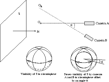
We define stereo visibility as an extension to the definition given above for the single camera. The direction of the cameras optical axis is known. Now we are only concerned with a set of non-coincident points that the two cameras may be placed at to simultaneously gain an unobstructed view of a given feature. To determine the visibility by a stereo pair of cameras the initial generation of the visibility cone is the same as for the single camera case. Once this has been done, it is then possible to remove all points corresponding to the position of one camera that do not guarantee that the features are also visible to the other camera.
To enforce the stereo constraint, it is necessary to remove all directions that differ
from the maximum deviation from the normal by an amount less than the separation of the
cameras. This is shown in figure 8, if the two cameras converge
at an angle ![]() then the visibility cone is offset by this value.
then the visibility cone is offset by this value.
Under certain circumstances it may not be possible to generate a representation of a
features stereo visibility. For example, when a face is only visible from directions that
all line on a plane normal to the plane on which the cameras lie. In this case an attempt
is made to resolve the problem by subdividing the face into smaller regions and then
testing the visibility of these regions independently.
We now present an outline of the algorithm that has been developed for building a view plan for astereo vision system. The algorithm is generic but can be customised for special application, such as object recognition or inspection, in which case special constraints are noted. Some of the algorithm before has been described previously in this paper, howvere note that additional steps are required specifically for the stereo problem. The output from the planner is a sequence of rotations interspersed by (where necessary for complete inspection) suitable repositioning instructions.
Another factor that can be considered when determining suitable weighting values are surface reflectance properties. Surfaces of certain types may scatter the laser light in such a way as to produce poor depth readings. There will also be problems if a face is imaged at angles close to the glancing angle.
Giving a feature a heavy weighting will cause the planner to try and choose a viewpoint such that it is imaged in a direction closer to its surface normal, i.e. its best view.
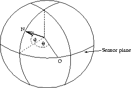
The normals can be represented by two angles, ![]() (figure 9).
(figure 9).
![]() represents the angle on the sensor plane with respect to the origin position.
represents the angle on the sensor plane with respect to the origin position.
![]() is the angle that a particular direction lies from the sensor plane. Since the
cameras are fixed, it is the value of
is the angle that a particular direction lies from the sensor plane. Since the
cameras are fixed, it is the value of ![]() that determines the best viewpoint. Hence
the centroid value that has been determined as the best viewpoint is translated into the
corresponding value of
that determines the best viewpoint. Hence
the centroid value that has been determined as the best viewpoint is translated into the
corresponding value of ![]() .
.
Repositioning the object to change the effective orientation of the sensor plane, ( i.e. relative to the object) involves rotating it with a robot arm. There is now the added complexity of having to deal with replacing the object in a stable orientation and re-registering the views. This is a slow process, i.e. actually moving the object and then registering the view, hence it is desirable that the inspection plan generated attempts to minimise these operations.
This applies equally to plan generation for other purposes, e.g. object recognition by model matching which requires that views of several different aspects are taken.
The problems of accuracy are important. The accuracy of the sensors, i.e. the resolution of the imaging system, is irrelevant to this stage. However the accuracy of the turntable and camera placement are. The planning system has been developed using a highly accurate commercial solid modeller. Therefore viewpoints selected assume that sensors can be placed to an equal level of accuracy. The accuracy of the turntable is known or can be calibrated, however there will be a finite and known number of possible rotations from the origin giving distinct views of the object. This suggests that there is a need to avoid viewpoints that all lie on a single plane opposing the cameras normal. These viewpoints would require the sensors to be placed to an extremely high degree of accuracy, any deviation from this position and direction would result in parts of the face being occluded to one of the cameras. To avoid having to deal with these conditions, such features are sub-divided into logical faces and treated separately.
In this section, examples are given that demonstrate the practical capability of the viewpoint planner. Results are given in two forms, graphical output from the solid modeller and real results from a vision acquisition system that uses a turntable and fixed camera to achieve multiple views. Space limitations prevent further discussion of results here. Results presented here demeonstrate that our planner can operate in a variety of domains -- for further results refer to [14].
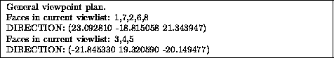
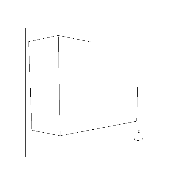
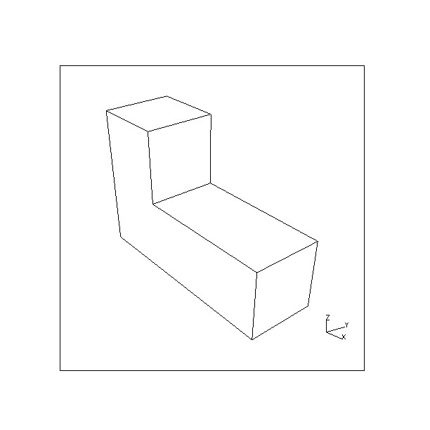
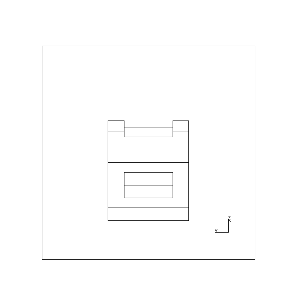
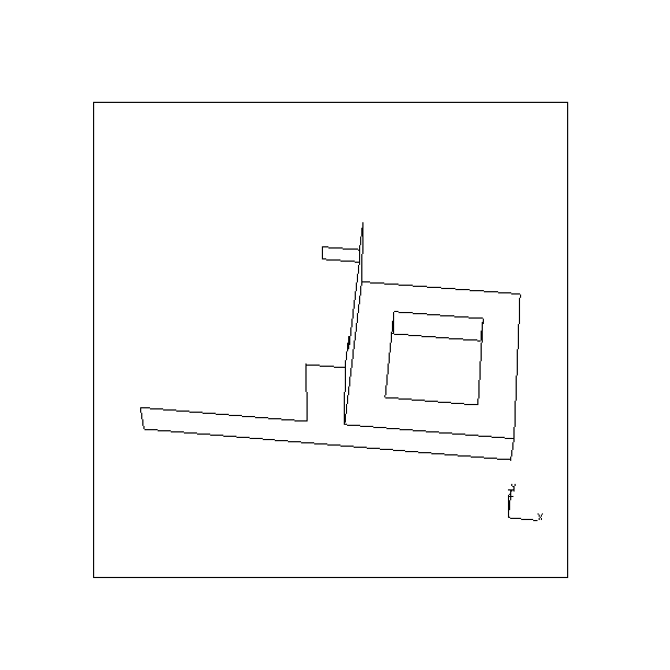
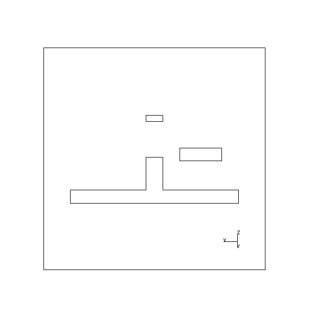
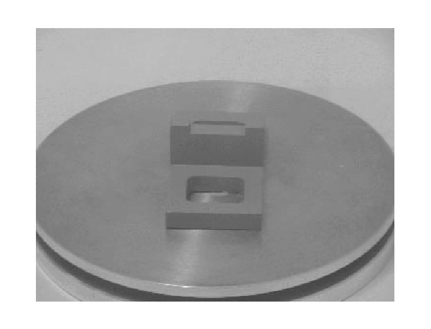
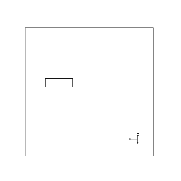
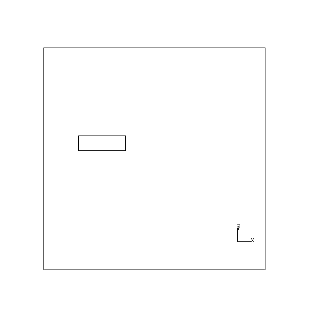
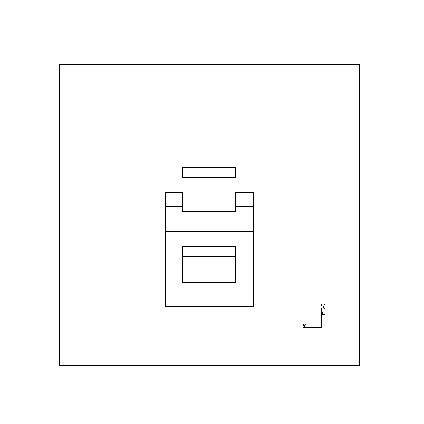
Results are given for the L-shaped block shown in Fig. 4. Table 3 shows part of the output from the viewpoint planner when no restrictions are applied to potential viewpoints. The object in this case hasn't been specified as lying on any surface and, hence, none of its faces are considered to be obscured by any part of its environment. Fig. 10 shows the two resultant views produced when the viewpoints are fed back into the solid modeller. By referring to Fig. 4, it can be seen that the viewpoints chosen give clear views of the faces indicated.
| View 1. To view faces 1,7,2,6,8 | View 2. To view faces 3,4,5 |
|---|---|
|
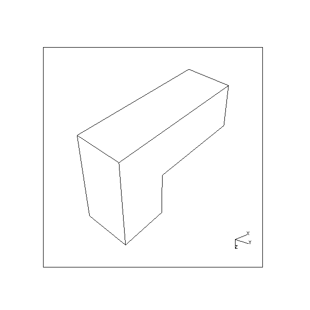 |
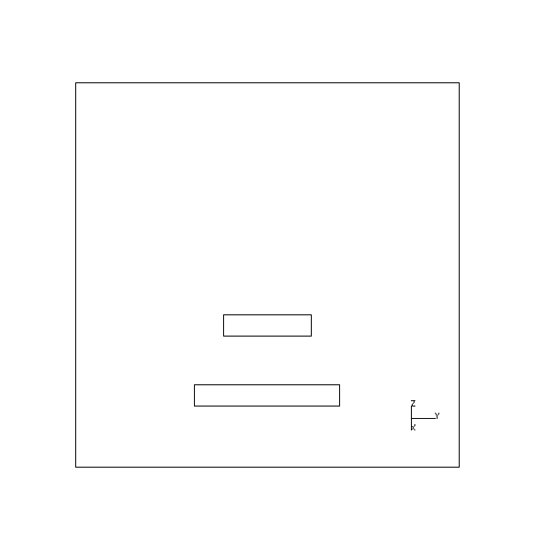
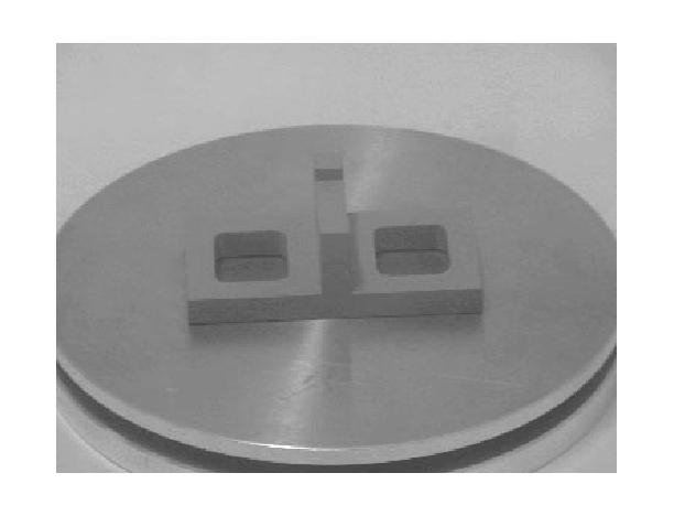
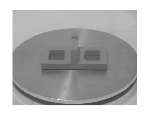
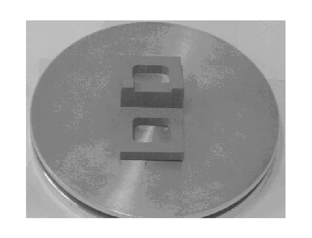
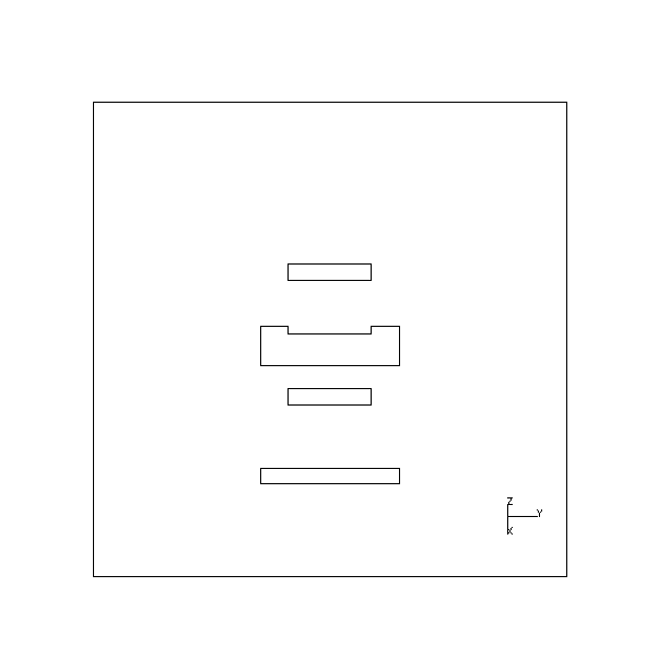
Fig. 11 shows the views chosen by the planner when possible viewpoints are restricted to a single degree of freedom relative to the object, i.e. suitable when a turntable is used to enable the acquisition of multiple views. In this instance, the object has been specified as resting on face 5, (i.e. the face with surface normal in the negative z direction), and the cameras pose is specified as being parallel and level with the turntable.
|
|
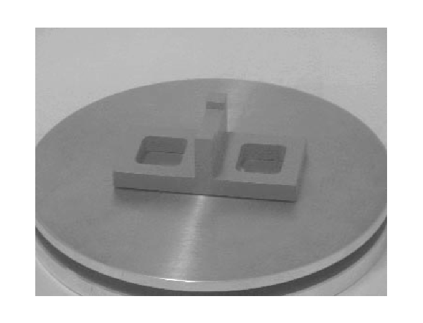
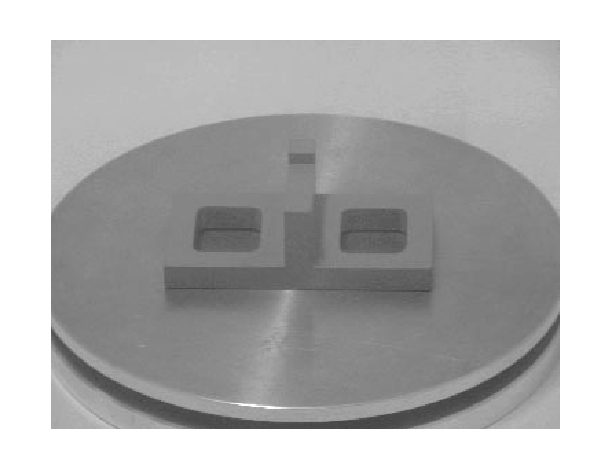
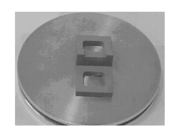
Fig. 12 shows the six views that were computed to view all possible faces of the object given the setup of the acquisition system used and a specified object pose. In this case, two faces besides the face obscured by the turntable are deemed to be impossible to see as a whole from any viewpoint given the current object and camera poses. Fig. 13 demonstrates how the problem of hidden faces can sometimes be overcome by changing camera pose. Here, the camera angle relative to the turntable has been increased and the planner now specifies the previously hidden faces to be suitable for viewing given the new camera pose and the pose of the object on the turntable.
| Actual View | Predicted modeler view | 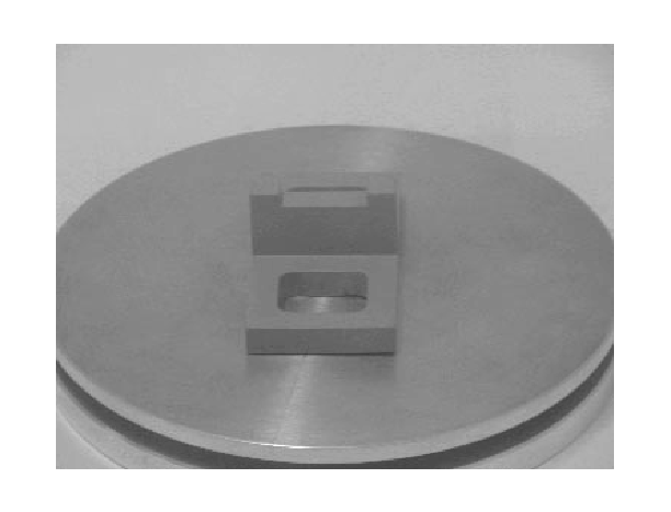 |
 |
|---|---|
 |
 |
 |
 |
 |
 |
 |
 |
 |
 |
| Actual View | Predicted modeler view |
|---|---|
 |
 |
 |
 |
In the experiment shown in Fig. 12 no constraint was imposed on the range of surface orientations that were chosen for viewing in a single image. Hence, in the second image a face has been chosen for viewing at a very oblique angle. However, in the second experiment, shown partly in Fig. 13, such a constraint was imposed. The face previously viewed at an oblique angle is now considered in a different view, shown in the second image, which results in a far better orientation relative to the camera.
Further details and results may be obtained from the following Research
Reports[14,15] and URLs:
http://www.cs.cf.ac.uk/Research/Rrs/1997/detail007.html,
http://www.cs.cf.ac.uk/Research/Rrs/1997/detail008.html
An algorithm has been presented that computes viewpoints suitable for viewing the complete surface area of an object. The approach taken to finding these viewpoints is based on constraint satisfaction. A graph representation is used to define the search space of solutions in which maximally connected subgraphs are sought since these correspond to faces that satisfy all constraints simultaneously and hence are suitable for viewing from a common viewpoint. The algorithm was first given in a more general form where viewing directions on the Gaussian sphere are sought. These are suitable for a work-cell in which a camera has been mounted on the end of a robot arm. An augmented algorithm was then given that is suitable for computing viewpoints in more restricted space, this would used when multiple views are obtained using a turntable. Practical results have been given that demonstrate the capability of the planner. Although not demonstarted here (due to space limitations) we can show that our planner is efficient in its operation ([14]). Our formulation of the search space is convenient and efficient, in comparison to other techniques, and has the advantage of manageable and known size of the search space prior to viewpoint deteremniation.