The active contour model described in Section ![]() is
an example of a model-driven segmentation technique. The Kalman
filter technique described in Section
is
an example of a model-driven segmentation technique. The Kalman
filter technique described in Section ![]() adds the
notion of statistical variation to the model-driven segmentation
process. In this section, I will introduce the Bayesian network
(BN) approach to segmentation. Bayesian networks are also referred to
as belief networks, probabilistic networks,
probabilistic belief networks (PBN), and probabilistic
causal networks. Since all of these terms can be used
interchangeably, I will refer to them as belief networks
throughout this dissertation. Regardless of the name, this approach
adds the dual notions of probability- and
utility-based decision making to the repertoire of segmentation
techniques. The belief network model makes decisions about how to
interpret probabilistic evidence (i.e., non-deterministic
information) to support or reject a hypothesis or
outcome. Outcomes that yield the highest expected utility
are chosen as the optimal solutions. With the belief network model,
the definition of expected utility incorporates all the probabilistic
uncertainty associated with the outcome, as well as the inherent
utility of the outcome. Utility can be defined in dimensions such as
monetary cost, entropy, or energy.
adds the
notion of statistical variation to the model-driven segmentation
process. In this section, I will introduce the Bayesian network
(BN) approach to segmentation. Bayesian networks are also referred to
as belief networks, probabilistic networks,
probabilistic belief networks (PBN), and probabilistic
causal networks. Since all of these terms can be used
interchangeably, I will refer to them as belief networks
throughout this dissertation. Regardless of the name, this approach
adds the dual notions of probability- and
utility-based decision making to the repertoire of segmentation
techniques. The belief network model makes decisions about how to
interpret probabilistic evidence (i.e., non-deterministic
information) to support or reject a hypothesis or
outcome. Outcomes that yield the highest expected utility
are chosen as the optimal solutions. With the belief network model,
the definition of expected utility incorporates all the probabilistic
uncertainty associated with the outcome, as well as the inherent
utility of the outcome. Utility can be defined in dimensions such as
monetary cost, entropy, or energy. ![]()
Many researchers have been using belief networks as a convenient mechanism for managing uncertainty in expert systems. Most of these expert systems to date have dealt with the tasks of classification or diagnosis in a temporally static problem domain. To a lesser extent, researchers have also been able to model dynamic properties using belief networks in an effort to simulate and predict the behavior of time-varying systems.
The idea of incorporating belief networks into this model-driven computer vision system was first proposed by Levitt and Binford [8]. The motivation for using belief networks was to make image interpretation insensitive to variations in structure, viewpoint, sensor type, shading, illumination, and obscuration [8]. Furthermore, real world image interpretation requires the ability to handle millions of features in a statistically efficient manner, using an accurate and rigorous mathematical model of uncertainty. According to Binford, relating image features such as step, delta, and slope discontinuities (i.e., boundaries and edges) to image structures and object models is a difficult problem.
Levitt and Binford argue that the belief network fits naturally into
the hierarchical image understanding model, where objects are composed
of parts and joints. Joints specify the relationships among parts,
which in turn are composed of subparts and joints. This recursive
relationship can be expressed in a directed acyclic graph (see
Section ![]() for a more detailed description of
directed graphs). Bayesian inference is used to accrue
evidence (i.e., observations) about the image in a mathematically
coherent framework. In this manner, a sufficient set of probabilistic
evidence, even if it is incomplete or ambiguous, can be amalgamated to
support or deny hypotheses about the objects in the image.
Competing hypotheses can be rank ordered by their overall probability,
or likelihood of occurrence.
for a more detailed description of
directed graphs). Bayesian inference is used to accrue
evidence (i.e., observations) about the image in a mathematically
coherent framework. In this manner, a sufficient set of probabilistic
evidence, even if it is incomplete or ambiguous, can be amalgamated to
support or deny hypotheses about the objects in the image.
Competing hypotheses can be rank ordered by their overall probability,
or likelihood of occurrence.
To briefly illustrate how a belief network can be used in model-based
vision, suppose we have two three-dimensional objects that we would
like to recognize from a photographic image: (a) a solid cube and (b)
a solid pyramid. The two DAGs shown in Figure ![]() represent the belief networks for these two objects. Let
represent the belief networks for these two objects. Let ![]() represent the hypothesis ``object is a cube,'' and
represent the hypothesis ``object is a cube,'' and ![]() represent the
hypothesis ``object is a pyramid.''
represent the
hypothesis ``object is a pyramid.''
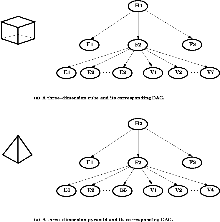
Figure: A simple belief network representation of two objects as
directed acyclic graphs (DAGs). The cube hypothesis (a) is
represented as an object with three visible faces, nine visible
edges, and seven visible vertices. The pyramid hypothesis (b)
is represented as an object with at most three visible faces,
six visible edges, and four visible vertices.
Given a photograph of a cube, we would expect to see at most three
faces, nine edges and seven vertices. For a three-sided pyramid, we
would expect to see at most three faces, six edges, and four vertices.
The DAG for the cube shows that ![]() gives rise to three faces (
gives rise to three faces ( ![]() ). In turn, each face gives rise to four edges (
). In turn, each face gives rise to four edges ( ![]() through
through ![]() ) and four vertices (
) and four vertices ( ![]() through
through ![]() ). By performing
statistical experiments, we can determine the probability of seeing
the faces under various lighting and viewing conditions. That is to
say, we can determine P(F|H) the probability of detecting a face,
given the type of object. Likewise, we can collect statistics on the
probabilities of seeing the edges and vertices P(E|F) and P(V|F)
given that we have seen a face. These statistics are called the
observed probabilities because they are based on what we can
observe from the image. What we would really like to know is the
inferred probability, that is, the probability that the face was
created a certain object. By using Baye's rule (also referred to as
Kolmogorov's theorem by statisticians), we can compute the inferred
probabilities. For example, the probability that a face was created
by a cube can be computed as
). By performing
statistical experiments, we can determine the probability of seeing
the faces under various lighting and viewing conditions. That is to
say, we can determine P(F|H) the probability of detecting a face,
given the type of object. Likewise, we can collect statistics on the
probabilities of seeing the edges and vertices P(E|F) and P(V|F)
given that we have seen a face. These statistics are called the
observed probabilities because they are based on what we can
observe from the image. What we would really like to know is the
inferred probability, that is, the probability that the face was
created a certain object. By using Baye's rule (also referred to as
Kolmogorov's theorem by statisticians), we can compute the inferred
probabilities. For example, the probability that a face was created
by a cube can be computed as
The inferred probability is now expressed in terms of the observed
probabilities ![]() ,
, ![]() , and
, and ![]() (where
(where ![]() means ``not''
means ``not'' ![]() , that is, the probability of seeing a face
given that the object is a pyramid).
, that is, the probability of seeing a face
given that the object is a pyramid). ![]() is also called the
prior probability of the cube hypothesis. In other words, it is
the overall probability that the object is a cube in the absence of
any other information. Statistically speaking,
is also called the
prior probability of the cube hypothesis. In other words, it is
the overall probability that the object is a cube in the absence of
any other information. Statistically speaking, ![]() is simply the
ratio of the cube population to the total population of objects.
is simply the
ratio of the cube population to the total population of objects.
In a similar manner, we can compute the probability that an edge was created by a face,
Strictly speaking, the probability of observing a face given an edge will vary depending on the number of edges that were detected. That is,
![]()
However, to reduce the complexity of the computations and the size of the statistical data gathering task, the assumption of conditional independence can be introduced. This assumption states that the probability of seeing one edge does not increase the probability of seeing another edge. As a result, the subscripts on the edges can be dropped,
![]()
Although it might be tempting to do so, it is not possible to compute
the probability of a hypothesis given an edge observation, ![]() ,
by simply multiplying P(H|F) by P(F|H). The computation of
,
by simply multiplying P(H|F) by P(F|H). The computation of
![]() is a non-trivial problem and was first solved by Pearl
(interested readers should consult [65] for a rigorous
derivation). There are many commercial software packages that will
compute inferred probabilities for belief networks using observed
statistical data.
is a non-trivial problem and was first solved by Pearl
(interested readers should consult [65] for a rigorous
derivation). There are many commercial software packages that will
compute inferred probabilities for belief networks using observed
statistical data.
In addition to observations about the presence of edges and vertices,
Binford and Levitt have proposed using relationships such as
parallelism, connectivity, and angular displacements as evidence in
the belief network. Furthermore, they have also proposed
parameterizing the observed probabilities as a function of the viewing
orientation. In this case, the observed probabilities would be
represented by probability distributions rather than by scalar
constants.![]() In
general, the computation of such probability distributions requires
quasi-invariant transformations to map random variables from the
measurement domain to the computation domain.
In
general, the computation of such probability distributions requires
quasi-invariant transformations to map random variables from the
measurement domain to the computation domain.
Several prototype systems have been built using the model-based belief
networks. In section ![]() I will describe a system
for segmenting two dimensional radiographic images. In
section
I will describe a system
for segmenting two dimensional radiographic images. In
section ![]() I will describe a complete vision system
for interpreting monocular greyscale images based on this technique.
I will describe a complete vision system
for interpreting monocular greyscale images based on this technique.