Next: Moment noise sensitivity
Up: Statistical moments - An
Previous: Image reconstruction
Relating Zernike and Cartesian moments
To help reduce computation complexity, it may prove useful to express the Zernike moments in terms of Cartesian moments. This removes the need for the polar mapping of the image, while also removing the dependence on the trigonometric functions. Alternatively, expressing Cartesian moments in this way would aid the selection of less correlated descriptors. This conversion can be achieved by slightly re-arranging the Zernike moment equation. If, as before, the Zernike polynomials are given by Equation 1.51 [22] and
the radial polynomials  are defined by Equation 1.52, re-arranging
  gives:
then substituting  and re-arranging again, produces:
 |
(71) |
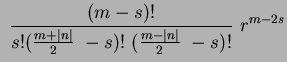
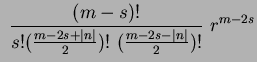
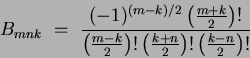
where:
 |
(72) |
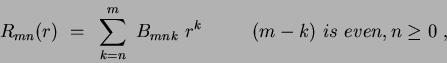
Using this manipulated form of the radial polynomials produces Zernike moment definitions (in continuous form) of:
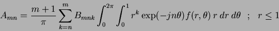 |
(73) |
which when translated to Cartesian coordinates is:
 |
(74) |
bounded by  and
and  .
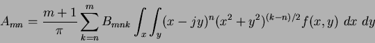
The double integral can now be expressed in terms of a series of summed Cartesian moments, of the form:
.
The double integral can now be expressed in terms of a series of summed Cartesian moments, of the form:
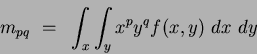 |
(75) |
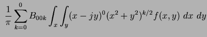
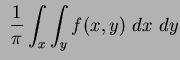
For example:
It must be noted that this comparison is only valid if the Cartesian moments are calculated on images confined to ![$[-1,1]$](img163.png) , which is due to the Zernike moments being calculated over the unit disc.
, which is due to the Zernike moments being calculated over the unit disc.
Next: Moment noise sensitivity
Up: Statistical moments - An
Previous: Image reconstruction
Jamie Shutler
2002-08-15