Hu invariant set

The non-orthogonal centralised moments are translation invariant and can be normalised with respect to changes in scale. However, to enable invariance to rotation they require reformulation. Hu [6] described two different methods for producing rotation invariant moments. The first used a method called principal axes, however it was noted that this method can break down when images do not have unique principal axes. Such images are described as being rotationally symmetric. The second method Hu described is the method of absolute moment invariants and is discussed here. Hu derived these expressions from algebraic invariants applied to the moment generating function under a rotation transformation. They consist of groups of nonlinear centralised moment expressions. The result is a set of absolute orthogonal (i.e. rotation) moment invariants, which can be used for scale, position, and rotation invariant pattern identification. These were used in a simple pattern recognition experiment to successfully identify various typed characters. 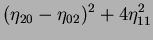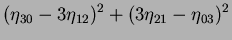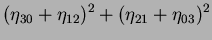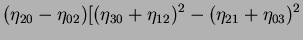They are computed from normalised centralised moments up to order three and are shown below$I_n$n$^{th}$ Hu invariant moment:

$$I_{1} = \eta_{20} + \eta_{02}$$ (37)

$$I_{2} = \mbox{} (\eta_{20} - \eta_{02})^{2} + 4\eta^2_{11}$$ (38)

$$I_{3} = \mbox{} (\eta_{30} - 3\eta_{12})^2 + (3\eta_{21} - \eta_{03})^2$$ (39)

$$I_{4} = \mbox{} (\eta_{30} + \eta_{12})^2 + (\eta_{21} + \eta_{03})^2$$ (40)

$$I_{5} = (\eta_{30} - 3\eta_{12})(\eta_{30} + \eta_{12})[(\eta_{30} + \eta_{12})^2 - 3(\eta_{21} + \eta_{03})^2] + (3\eta_{21}$$ (41)

$$- \eta_{03})(\eta_{21} + \eta_{03})[3(\eta_{30} + \eta_{12})^2 - (\eta_{21} + \eta_{03})^2]$$

$$I_{6} = \mbox{} (\eta_{20} - \eta_{02})[(\eta_{30} + \eta_{12})^2 - (\eta_{21} + \eta_{03})^2$$ (42)

$$+ 4\eta_{11}(\eta_{30} + \eta_{12})(\eta_{21} + \eta_{03})]$$

Finally a skew invariant, to help distinguish mirror images, is: [RBF note: original paper has "...eta_03)^2]-(eta_30-3*eta_12)(..."]

$$I_{7} = (3\eta_{21} - \eta_{03})(\eta_{30} + \eta_{12})[(\eta_{30} + \eta_{12})^2 - 3(\eta_{21}$$

$$+ \eta_{03})^2] + (\eta_{30} - 3\eta_{12})(\eta_{21} + \eta_{03})[3(\eta_{30}$$ (43)

$$+ \eta_{12})^2 - (\eta_{21} + \eta_{03})^2]$$

These moments are of finite order, therefore, unlike the centralised moments they do not comprise a complete set of image descriptors, [8]. However, higher order invariants can be derived, [2,6]. It should be noted that this method also breaks down, as with the method based on the principal axis for images which are rotationally symmetric as the seven invariant moments will be zero [12].