In an image processing context, the histogram of an image normally refers to a histogram of the pixel intensity values. This histogram is a graph showing the number of pixels in an image at each different intensity value found in that image. For an 8-bit grayscale image there are 256 different possible intensities, and so the histogram will graphically display 256 numbers showing the distribution of pixels amongst those grayscale values. Histograms can also be taken of color images --- either individual histograms of red, green and blue channels can be taken, or a 3-D histogram can be produced, with the three axes representing the red, blue and green channels, and brightness at each point representing the pixel count. The exact output from the operation depends upon the implementation --- it may simply be a picture of the required histogram in a suitable image format, or it may be a data file of some sort representing the histogram statistics.
The operation is very simple. The image is scanned in a single pass and a running count of the number of pixels found at each intensity value is kept. This is then used to construct a suitable histogram.
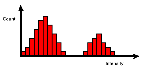
Histograms have many uses. One of the more common is to decide what
value of threshold to use when converting a grayscale image to a
binary one by thresholding. If the image is suitable
for thresholding then the histogram will be bi-modal --- i.e. the
pixel intensities will be clustered around two well-separated values.
A suitable threshold for separating these two groups will be found
somewhere in between the two peaks in the histogram. If the
distribution is not like this then it is unlikely that a good
segmentation can be produced by thresholding.
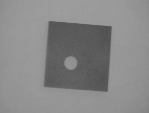
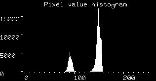
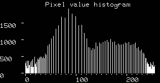
The intensity histogram for the input image
is
The object being viewed is dark in color and it is placed on a light background, and so the histogram exhibits a good bi-modal distribution. One peak represents the object pixels, one represents the background. The histogram
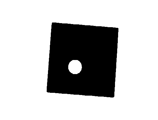
is the same, but with the y-axis expanded to show more detail. It is clear that a threshold value of around 120 should segment the picture nicely, as can be seen in
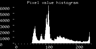
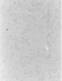
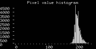
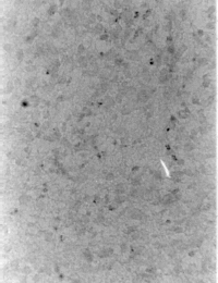
The histogram of image
is
This time there is a significant incident illumination gradient across the image, and this blurs out the histogram. The bi-modal distribution has been destroyed and it is no longer possible to select a single global threshold that will neatly segment the object from its background. Two failed thresholding segmentations are shown in
and
using thresholds of 80 and 120, respectively.
It is often helpful to be able to adjust the scale on the y-axis of the histogram manually. If the scaling is simply done automatically, then very large peaks may force a scale that makes smaller features indiscernible.
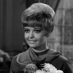
The histogram is used and altered by many image enhancement operators. Two operators which are closely connected to the histogram are contrast stretching and histogram equalization. They are based on the assumption that an image has to use the full intensity range to display the maximum contrast. Contrast stretching takes an image in which the intensity values don't span the full intensity range and stretches its values linearly. This can be illustrated with
Its histogram,
shows that most of the pixels have rather high intensity values. Contrast stretching the image yields
which has a clearly improved contrast. The corresponding histogram is
If we expand the y-axis, as was done in
we can see that now the pixel values are distributed over the entire intensity range. Due to the discrete character of the pixel values, we can't increase the number of distinct intensity values. That is the reason why the stretched histogram shows the gaps between the single values.
The image
also has low contrast. However, if we look at its histogram,
we see that the entire intensity range is used and we therefore cannot apply contrast stretching. On the other hand, the histogram also shows that most of the pixels values are clustered in a rather small area, whereas the top half of the intensity values is used by only a few pixels. The idea of histogram equalization is that the pixels should be distributed evenly over the whole intensity range, i.e. the aim is to transform the image so that the output image has a flat histogram. The image
results from the histogram equalization and
is the corresponding histogram. Due to the discrete character of the intensity values, the histogram is not entirely flat. However, the values are much more evenly distributed than in the original histogram and the contrast in the image was essentially increased.
You can interactively experiment with this operator by clicking here.
R. Boyle and R. Thomas Computer Vision: A First Course, Blackwell Scientific Publications, 1988, Chap. 4.
E. Davies Machine Vision: Theory, Algorithms and Practicalities, Academic Press, 1990, Chap. 4.
A. Marion An Introduction to Image Processing, Chapman and Hall, 1991, Chap. 5.
D. Vernon Machine Vision, Prentice-Hall, 1991, p 49.
Specific information about this operator may be found here.
More general advice about the local HIPR installation is available in the Local Information introductory section.
©2003 R. Fisher, S. Perkins,
A. Walker and E. Wolfart.
![]()