The Bio-PEPA Eclipse Plug-inUser Manual: Syntax Example: Bidirectional Transportation, Modifier

A.10 Syntax Example: Bidirectional Transportation, Modifier

The model shown in Table 6 has two locations, the parent location which is called $main$ and is a membrane, and the $child$ location which is a compartment enclosed by the membrane (see Figure 77). In the definition of location $child$ , the $type$ is not declared as it defaults to compartment. The model contains two species $A$ and $B$ . Species $A$ is originally located both in membrane $main$ ( $A@main$ ) and in compartment $child$ ( $A@child$ ). Species $A$ is involved in the $\mathit{tr}$ reaction, which is a bidirectional transportation ( $\leftrightarrow$ , <->) reaction representing the movement of species $A$ from membrane $main$ to compartment $child$ and vice versa. The $\mathit{tr}$ reaction is described by mass-action kinetics ( $fMA(r_{1})$ ), where $r_1$ is a kinetic parameter that has been given the constant value of 0.01 (see section A.4 for more information on mass-action kinetics). Moreover, species $A@child$ and $B$ are involved in the $\mathit{re}$ reaction, which takes plase in compartment $child$ . The rate of $\mathit{re}$ is governed by kinetic parameter $r_{2}$ which has been given the constant value of 0.01. The rate of $\mathit{tr}$ also depends on the quantity of $A$ available in compartment $child$ ( $A@child$ ). The quantity of species $B$ that is produced is located in $child$ , where $\mathit{re}$ takes place.

In the species components definition, the general modifier operator ( $\odot$ , (.)) is used for transportation as, while the levels of species $A$ in the two locations change, the overall amount does not.

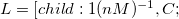
The Outline View of the model can be seen in Figure 79.

The Bio-PEPA syntax	`//The Bio-PEPA plugin syntax`
Locations:	`//Locations`
$L = [ child : 1 (nM)^{-1}, C;$	`location child in main : size = 1;`
$\; \; \; \; \; \; \; \; main : 2 (nM)^{-1}, M;]$	`location main : size = 2, type = membrane;`
$\text{[math]}$
Parameter Definitions	`//Parameter Definitions`
$r_1 = 0.01;$	`r1 = 0.01;`
$r_2 = 0.01;$	`r2 = 0.01;`
$\text{[math]}$
	`//Variables for the species initial populations`
	`Am = 100;`
	`Ac = 100;`
	`B = 0;`
$\text{[math]}$
Functional Rates	`//Functional Rates`
$f_{tr} = [fMA(r_1)];$	`tr = [fMA(r1)];`
$f_{re} = [ r_2 * A@child];$	`re = [ r2 * A@child];`
$\text{[math]}$
Species Components	`//Species Components`
$A \rmdef (tr[main \leftrightarrow child], 1) \modifier A + (re, 1) \reactant A$	`A = tr[main<->child] (.) A + re << A@child;`
$B \rmdef (re, 1) \product B$	`B = re >>;`
$\text{[math]}$
Model Component	`//Model Component`
$A@main[100] \sync{tr} A@child[100] \sync{re} B@child[0]$	`A@main[Am]<tr>A@child[Ac]<re>B@child[B]`

Table 6: Bio-PEPA mathematical syntax and Bio-PEPA Eclipse Plug-in syntax for the Bidirectional Transportation model

$\includegraphics[scale=0.5]{screenshots/screenshots/bitranspoutline}$

Figure 79: The Outline View of the Bidirectional Transportation model