Hao Tang 唐顥
Speech Features
In this post, I will give a quick overview of the commonly used operations, such as Fourier transform, windowing, and Mel filters, for processing speech signals.
Waveform
A wave file is simply a sequence of amplitudes of the sound wav. Typical numbers of measurements range from 8000Hz (i.e., 8000 samples per second) to 48000Hz. We can plot the amplitudes against the time axis. An example of waveform and its corresponding wave file are shown in the figure below.

To see the characteristic of speech, we need to zoom in and take a closer look at the sound wave. Below is a more detailed plot from 0.2s to 0.35s.

Here are a few quick observations.
Speech is not stationary. Segment $a$ and segment $b$ clearly looks different.
-
Some parts of speech are periodic. We can clearly see repeated patterns in segment $b$. In fact, there are around 12 peaks within the 0.05s between 0.30s and 0.35s, so the frequency is about 240Hz.
Partly because a large part of the speech signal is periodic and partly because human ears are great frequency analyzers, Fourier transform, a mathematical tool that decomposes a signal into sinusoids, have been used to analyze the frequency components of speech. We will talk about discrete Fourier transform next and come back to the issue of non-stationarity.
Discrete Fourier Transform
A signal is a sequence of complex numbers. For example, the sequence of amplitudes we just saw is a signal. The numbers are indexed, usually by time. For a signal $x$, we will use $x[t]$ to denote the number at time $t$. For our purposes, we will assume $t \in \mathbb{Z}$, and this type of signal is called discrete-time signal, or discrete signal for short.
A discrete Fourier transform (DFT) is defined as \begin{align} X[n] = \sum_{t=0}^{N-1} x[t] e^{-j \frac{2 \pi n}{N}t}, \end{align} for $n = 0, \dots, N-1$, where $j = \sqrt{-1}$ and $N$ is the number of samples in $x$. To get some intuition for understanding DFT, we will look at the properties of this operation.
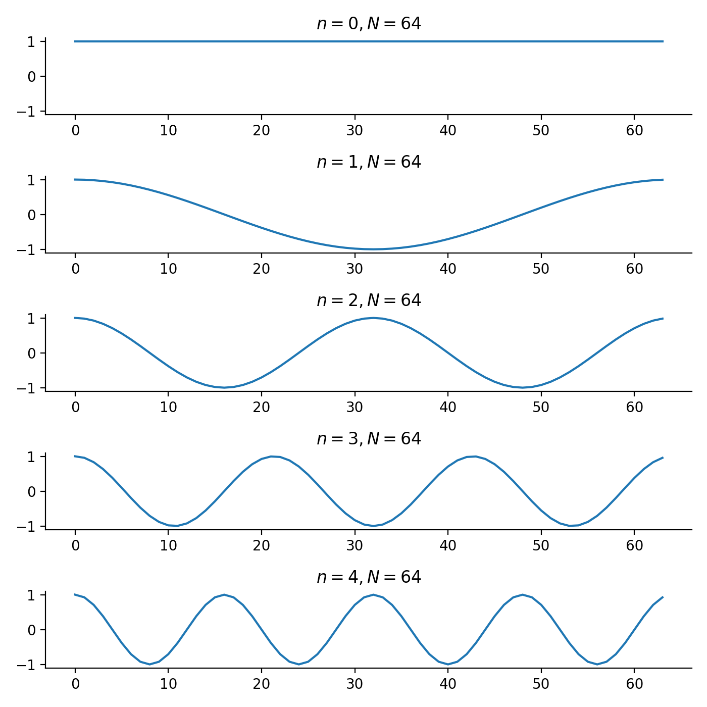
We can write the DFT as \begin{align} X[n] = \begin{bmatrix} 1 & e^{-j \frac{2 \pi n}{N} 1} & \cdots & e^{-j \frac{2 \pi n}{N} (N-1)} \end{bmatrix} \begin{bmatrix} x[0] \\ x[1] \\ \vdots \\ x[N-1] \end{bmatrix} = v_n^* x, \end{align} so DFT is simply a complex dot product, where $u^*$ is the conjugate transpose of the vector $u$ and $v_n = \begin{bmatrix} 1 & e^{j \frac{2 \pi n}{N}} & \cdots & e^{j \frac{2 \pi n}{N} (N-1)} \end{bmatrix}$. Note that \begin{align} v_n^* v_m = \sum_{t=1}^N e^{j \frac{2 \pi (m-n)}{N} t} = \begin{cases} \frac{1 - \exp\left( \frac{j 2\pi (m-n)}{N} N \right)}{1 - \exp \left( j\frac{2 \pi (m-n)}{N} \right)} = 0 & \text{if $m \neq n$} \\ N & \text{if $m=n$} \end{cases}. \end{align} In other words, $v_n$ and $v_m$ are orthogonal if $m \neq n$, and the set of vectors $V = \{v_1 / \sqrt{N}, \dots, v_N / \sqrt{N}\}$ is an orthonormal basis. The basis $V$ is called the Fourier basis, and we can interpret DFT as a change of coordinates.
Each basis element can be treated as a signal. Specifically, $v_n[t] = e^{j 2\pi n t / N}$. Recall that $e^{j\omega t} = \cos(\omega t) + j \sin(\omega t)$. Below shows the real part of a few basis elements. We can see that $v_n$ is a signal of frequency $n / N$.
Since $X[n] = v_n^* x$, we can intuitively think of $X[n]$ as a measure of how similiar $x$ is to $v_n$. In fact, X[n] is exactly the amount of $v_n$ needed to constitute $x$. To see this, because DFT is a change of coordinates, we can also convert $X$ back to $x$ with \begin{align} x[t] = \frac{1}{N} \sum_{n=0}^{N-1} X[n] e^{j \frac{2 \pi n}{N} t} \end{align} In other words, we can write $x$ as a weighted combination of complex sinusoids, The value $X[n]$ it is the weight of the complex sinusoid $v_n$ that constitutes $x$.
Below is an example of reconstructing the original signal by adding complex sinusoids of increasing frequency.
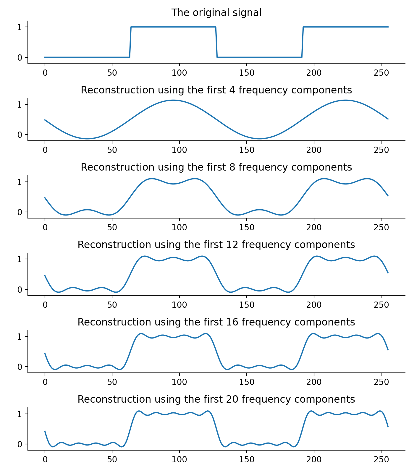
Typically, the weighted combination of low-frequency complex sinusoids is responsible for reconstructing the overall shape of the signal, and the high-frequency complex sinusoids is responsible for reconstructing the fine details of signal. We will make use of this property later when we talk about cepstrum coefficients.
There are various names to refer to $X$. The values $X[0], X[1], \dots, X[N-1]$ are sometimes called frequency components of $x$. The vector $X$ is also called the spectrum of $x$, and we will also refer to DFT more broadly as spectral analysis.
Windowing
Recall that speech is not stationary. If we want to know the content of speech that changes over time, instead of doing spectral analysis over the entire utterance, it is better to do the analysis over small periods of time and do it frequently. To achieve this, we create a window, and only focus on the samples within the window.
There are various types of window functions. The simplest window function is the rectangular window defined as \begin{align} w[t] = \begin{cases} 1 & \text{if $0 \leq t \leq a$,} \\ 0 & \text{otherwise,} \end{cases} \end{align} where the window is of size $a$. We can shift the window to a time we want to focus on. For example, if \begin{align} y[t] = x[t] w[t - b], \end{align} we have a window centered at time $b$ and the signal $y$ contains samples of $x$ between time $b$ and time $b + a$.
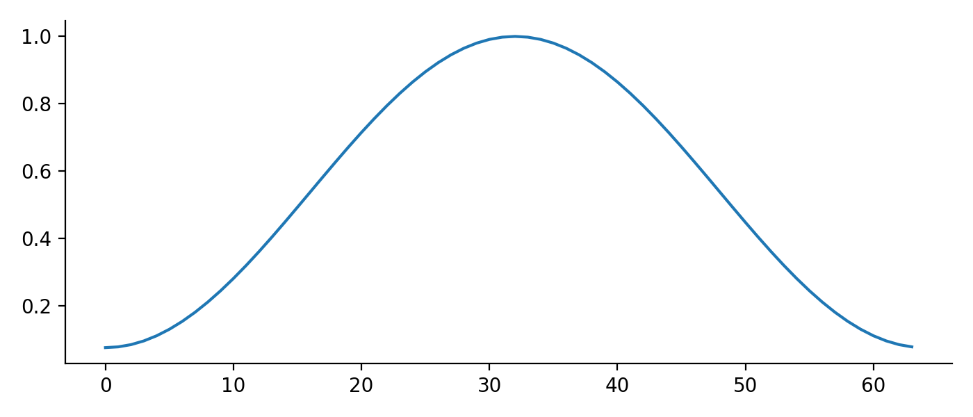
The window function typically used in speech processing is the Hamming window \begin{align} w[t] = 0.54 - 0.46 \cdot \cos\left(\frac{2\pi t}{N} \right). \end{align} Below is a plot of a Hamming window of size 64.
Choosing what window function to use is an art, and I will not attempt to justify the use of a particular window function. For reproducibility, we will follow the convention and use the Hamming window to process speech.
The last question is how often we should do spectral analysis, and this is called the hop length. Simply put, we perform spectral analysis every $h$ samples if the hop length is $h$. We will come back to this in the following section.
Spectrogram
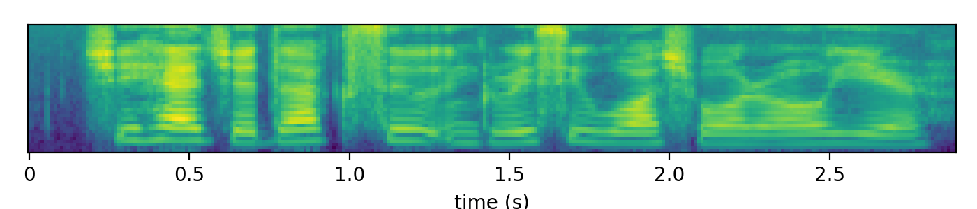
We want to analyze speech frequently over small periods of time, and we have the tools ready to realize this. The goal can now be translated into performing spectral analysis with a small hop length and a small window length. Each analysis results in a vector of complex numbers. The information in magnitudes suffices for many speech applications, so we leave out the phase away for now. We pack the vectors of magnitudes into a matrix, and that matrix is called a spectrogram.
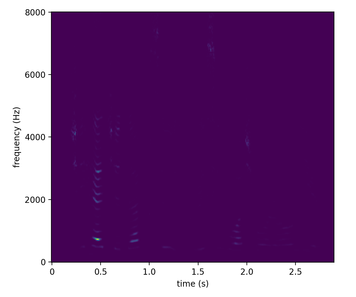
Below is an example spectrogram of the waveform we looked at the beginning of this post, with a hop length of 10ms and a window length of 25ms.
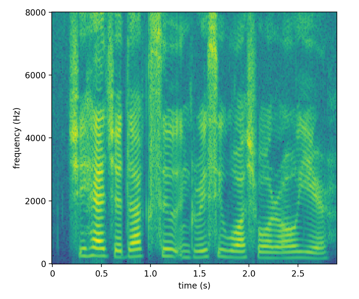
The magnitudes has a large dynamic range, and is difficult to see the details. To compress the dynamic range and given that the magnitudes are always nonnegative, we take elementwise the log and arrive at the following figure.
We can play around with the hop length and window length. Below is the spectrogram with a hop length of 1ms and a window length of 6ms. (Technically, I am computing DFT using 1024 basis elements for this particular example. Given such a small window, we need to pad zeros at the end.)
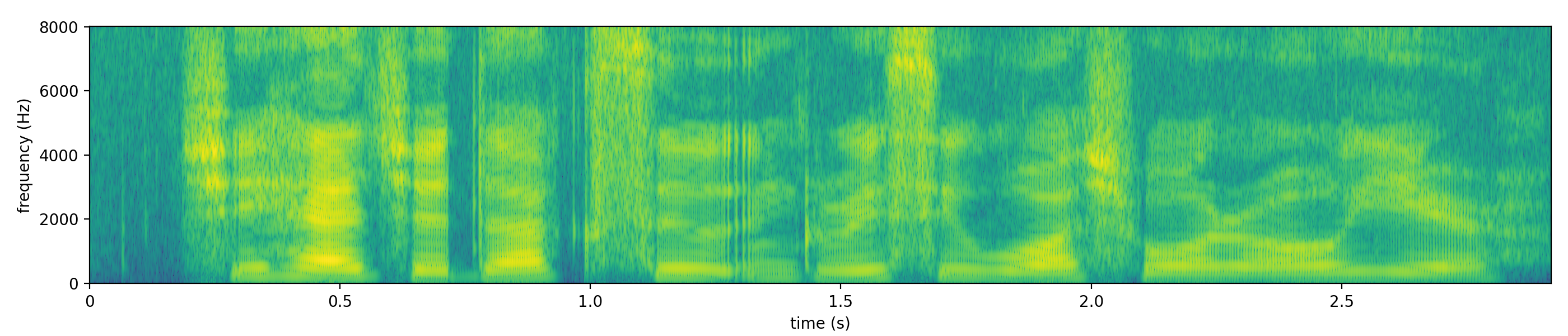
We will not discuss what the patterns are at this point, but it suffices to say that there are patterns in the spectrogram and the patterns are more directly visible compared to the waveforms.
Mel filters
The physical properties of sound correlates well with how one perceives it. For example, if the power of the sound is larger, then one would hear the sound louder; if the frequency of the sound is higher, then one would hear the sound higher. What is interesting is that the scale is not linear. Experiments have been done to map out the scale, and there exist many different scales. The most commonly used one in speech processing is the Mel scale where the relation ship between the perceived frequency and the physical frequency is described as \begin{align} m = 1127 \log \left( 1 + \frac{f}{700} \right). \end{align}
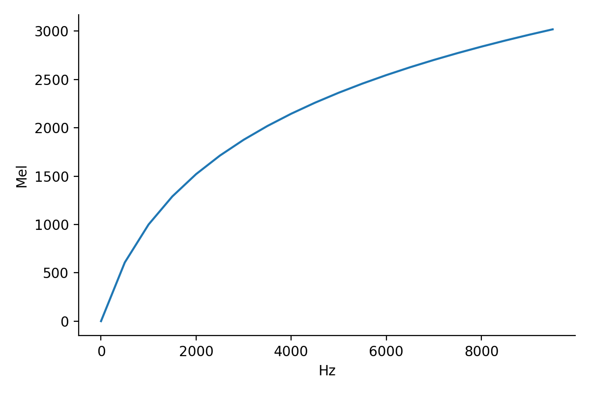
Figure 9 shows the Mel scale. The key property is that the perceived frequency is more sensitive at low frequencies and less sensitive at high frequencies.
Besides the nonlinear scale in frequency, human hearing has another interesting property: the inability to tell two different tones when the frequencies of the two tones are close. The minimum amount of frequency difference needed to tell the two tones is called the critical band. The bandwidth also depends on the frequency: the higher the frequency, the larger the bandwidth. This again shows that human ears are more sensitive in low frequencies and less sensitive in high frequencies.
The concept of critical bands can be implemented with a filter bank. A filter is a vector that is applied to the frequency components of a signal. For example, if \begin{align} Y[n] = X[n] \phi[n], \end{align} we say that the vector $\phi$ is a filter and it is applied to the frequency components $X$ of the signal $x$ to get the frequency components $Y$ of the signal $y$. Elementwise multiplication is commonly used for applying filters, but we are not restricted to this particular operation. A filter bank is simply a set of filters.
A filter is like any other frequency components, and we can plot them on the frequency axis. Figure 10 shows one example, and it is a vector \begin{align} \begin{bmatrix} 0 & \cdots & 0 & 0.056 & 0.121 & 0.185 & \cdots 0.183, 0.122, 0.061 \end{bmatrix} \end{align} with zeros before 7000Hz, linearly increasing values after 7000Hz, and linearly decreasing values after around 7500Hz. (Note that the filter looks like an isosceles triangle, but it is not.)
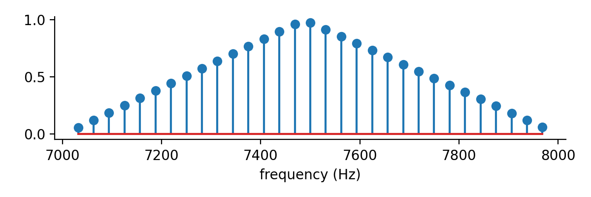
The triangular filter in Figure 10 is one approach to implementing a critical band, where the frequency components away from a frequency around 7500Hz are attenuated. In fact, it is one of the filters in the Mel filter bank. Figure 11 shows the Mel filter bank.
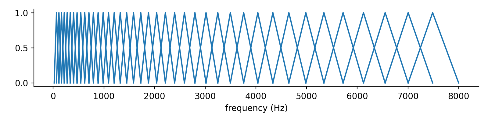
The filter bank is constructed as follows. First, we have a set of values equally spaced in Mel scale. Take any contiguous three values, convert them back to regular frequencies, and linearly interpolating the filter values between the frequencies.
To apply the Mel filter bank, instead of elementwise multiplication, the common approach is to do dot product. Specifically, suppose we have $K$ Mel filters $\phi_1, \phi_2, \dots, \phi_K$. The result of applying the $k$-th Mel filter is \begin{align} Y[k] = \sum_{n=0}^{N-1} X[n] \phi_k[n]. \end{align} Applying the entire filter bank simply becomes a matrix-vector multiplication.
If we apply a Mel filter bank of 40 Mel filters, evenly spaced from 20Hz to 8000Hz, to the spectrogram in Figure 7, we have the Mel spectrogram in Figure 12. This is the dominant representation used for speech recognition nowadays.