Hao Tang 唐顥
Gaussian Mixture Models
Recall from last time that frames of different phones look different, and we quantify the difference with $\ell_2$ norm. Figure 1 and 2 show how the frames differ for different phones, but notice that frames within the phone [u] also exhibits certain variation. In other words, the frames within a phone differ less, while frames from different phones differ more. In this post, we will formalize what it means for frames to differ less or to differ more, and use this basic observation to cluster frames.

Gaussian Mixture Models (GMM)
To model the variation of frames of a specific phone, we can (crudely) assume the variation behaves like a Gaussian. Formally, suppose $\pi = (\pi_1, \dots, \pi_K)$ defines the probability of choosing a class from $K$ classes. In other words, $0 \leq \pi_k \leq 1$, and $\sum_{k=1}^K \pi_k = 1$. We can think of the $K$ classes as phones, but the classes do not necessarily need to correspond to phones. Suppose we have $N$ data points $x_1, \dots, x_N$, and they are produced by the generative process \begin{align} z_n & \sim \text{Categorical}(\pi) \\ x_n & \sim \mathcal{N}(\mu_{z_n}, \Sigma_{z_n}) \end{align} for $n = 1, \dots, N$. In words, for the $n$-th sample, we first choose a class based on $\pi$, call it $z_n$, and choose a frame from a Gaussian centered at $\mu_{z_n}$ with covariance $\Sigma_{z_n}$. If you are not familiar with the notation, $z_n \sim \text{Categorical}(\pi)$ is a fancy way of saying \begin{align} p(z_n) = \pi_{z_n}, \end{align} and $x_n \sim \mathcal{N}(\mu_{z_n}, \Sigma_{z_n})$ is a fancy way of saying \begin{align} p(x_n | z_n) = \frac{1}{(2\pi)^{d/2}|\Sigma_{z_n}|^{1/2}} \exp \left(-\frac{1}{2} (x_n - \mu_{z_n})^\top \Sigma^{-1}_{z_n} (x_n - \mu_{z_n}) \right), \end{align} where $d$ is the dimension of $x_n$'s. By the definition of conditional probability, \begin{align} p(x_n, z_n) &= p(x_n|z_n) p(z_n) \\ &= \pi_{z_n}\frac{1}{(2\pi)^{d/2}|\Sigma_{z_n}|^{1/2}} \exp \left(-\frac{1}{2} (x_n - \mu_{z_n})^\top \Sigma^{-1}_{z_n} (x_n - \mu_{z_n}) \right). \end{align} This is known as Gaussian mixture models, and the parameters are the means $\mu_1, \dots, \mu_K$ and the covariance matrices $\Sigma_1, \dots, \Sigma_K$.
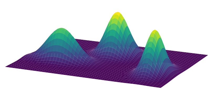
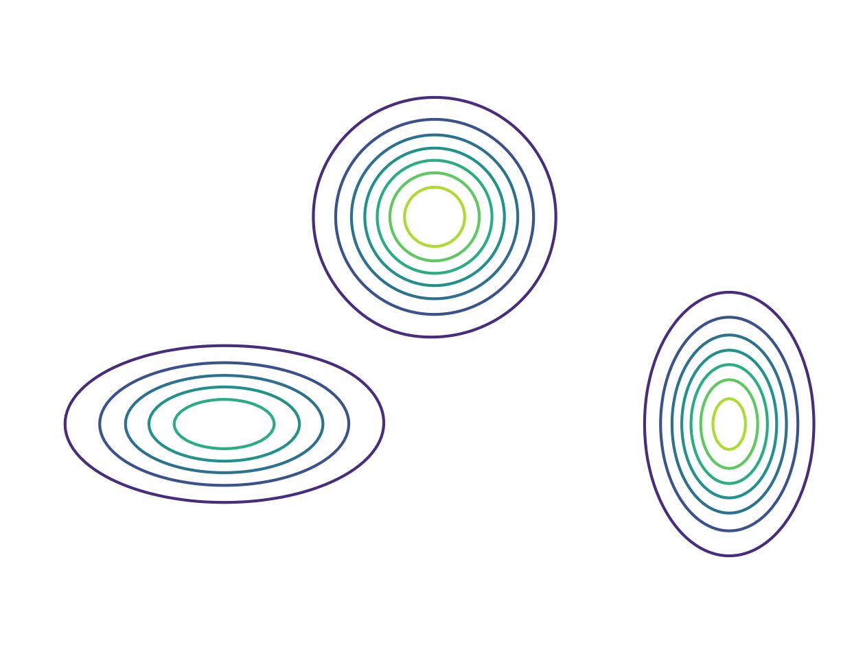
An example GMM with $d=2$ and $K=3$ is shown in Figure 3. Another common way to visualize the probability density is to use contours, as shown in Figure 4.
Maximum Likelihood Estimation
Note that the outcome of the generative process is a set of independent vectors $\{x_1, \dots, x_N\}$, and we do not get to access or to observe the $z_n$'s, i.e., the classes. Given the set of independent samples $\{x_1, \dots, x_N\}$, we can ask what the most likely set of means and covariance matrices is. This is called the maximum likelihood estimation of the parameters. Formally, the log likelihood of the means and covariance matrices is \begin{align} \log \prod_{n=1}^N p(x_n) &= \sum_{n=1}^N \log p(x_n) \\ &= \sum_{n=1}^N \log \sum_{z_n=1}^K p(x_n, z_n) \\ &= \sum_{n=1}^N \log \sum_{z_n=1}^K p(z_n) p(x_n | z_n) \\ &= \sum_{n=1}^N \log \sum_{z_n=1}^K \pi_{z_n} \frac{1}{(2\pi)^{d/2} |\Sigma_{z_n}|^{1/2}} \exp \left(-\frac{1}{2} (x_n - \mu_{z_n})^\top \Sigma_{z_n}^{-1} (x_n - \mu_{z_n}) \right) \\ &\triangleq L(\theta), \end{align} where $\theta = \{\mu_1, \dots, \mu_K, \Sigma_1, \dots, \Sigma_K\}$. The maximum likelihood estimation of the means and covariance matrices is \begin{align} \hat{\theta} = \operatorname*{\arg\!\!\max}_\theta L(\theta). \end{align} In principle, $L$ is nothing but a real-valued function, and can be optimized with any off-the-shelf optimization algorithm, such as gradient descent. However, below we will take a different approach in optimizing the objective function $L$.
A Variational Lower Bound
We start with the log likelihood, and let \begin{align} L &= \sum_{n=1}^N \log p_\theta(x_n) \\ &= \sum_{n=1}^N \log \sum_{z_n=1}^K p_\theta(x_n, z_n) \\ &= \sum_{n=1}^N \log \sum_{z_n=1}^K q_n(z_n) \frac{p_{\theta}(x_n, z_n)}{q_n(z_n)} \\ &= \sum_{n=1}^N \log \mathbb{E}_{z_n \sim q_n} \left[\frac{p_{\theta}(x_n, z_n)}{q_n(z_n)}\right], \end{align} where $q_n(z)$ is an arbitrary distribution with $0 \leq q_n(z) \leq 1$ and $\sum_{z=1}^K q_n(z) = 1$. Note that the dependency of $\theta$ is made explicit. Now we can apply Jensen's inequality to swap the log and the expectation, and get \begin{align} L &= \sum_{n=1}^N \log \mathbb{E}_{z_n \sim q_n} \left[\frac{p_{\theta}(x_n, z_n)}{q(z_n)}\right] \\ &\geq \sum_{n=1}^N \mathbb{E}_{z_n \sim q_n} \left[ \log \frac{p_{\theta}(x_n, z_n)}{q(z_n)} \right] \\ &= \sum_{n=1}^N \sum_{z_n=1}^K q_n(z_n) \log \frac{p_{\theta}(x_n, z_n)}{q_n(z_n)} \\ &= \sum_{n=1}^N \sum_{z_n=1}^K q_n(z_n) \log p_{\theta}(x_n, z_n) + \sum_{n=1}^N H(q_n) \\ &\triangleq \text{ELBO}(q, \theta) \end{align} where $q = \{q_1, \dots, q_N\}$, $H(q_n)$ is the entropy of $q_n$, and as before $\theta = \{\mu_1, \dots, \mu_K, \Sigma_1, \dots, \Sigma_K\}$. The penultimate line is commonly known as the variational lower bound or the evidence lower bound (ELBO).
In short, the inequality \begin{align} L(\theta) \geq \text{ELBO}(q, \theta) \end{align} holds for any $q$ and any $\theta$. Since ELBO is a lower bound of the likelihood, the hope is that if we attempt to increase ELBO, the likelihood would be increased.
Expectation Maximization (EM)
Given the variational lower bound of the likelihood, a simple strategy is to do alternating maximization where we iterate between optimizing $q$ with $\theta$ fixed and optimizing $\theta$ with $q$ fixed. Formally, the $t$-th iteration of the algorithm we perform \begin{align} q_{t} &= \operatorname*{\arg\!\!\max}_q \text{ELBO}(q, \theta_{t-1}) \\ \theta_{t} &= \operatorname*{\arg\!\!\max}_\theta \text{ELBO}(q_t, \theta). \end{align} The first and the second step are typically called the E-step and the M-step, respectively.
The first thing to note is that the posterior probability $p(z_n | x_n)$ is actually the optimal $q_n$ we can attain. To show this, we can simply plug in $q_n(z_n) = p(z_n | x_n)$ to ELBO and get \begin{align} \sum_{n=1}^N \sum_{z_n=1}^K p(z_n | x_n) \log \frac{p(x_n, z_n)}{p(z_n | x_n)} &= \sum_{n=1}^N \sum_{z_n=1}^K p(z_n | x_n) \log p(x_n) \\ &= \sum_{n=1}^N \log p(x_n) \sum_{z_n=1}^K p(z_n | x_n) \\ &= \sum_{n=1}^N \log p(x_n) = L. \end{align} In other words, the inequality $L(\theta) \geq \text{ELBO}(q, \theta)$ becomes equality when $q_n(z_n) = p_\theta(z_n | x_n)$.
For Gaussian mixture models, the posterior of the $n$-th sample can be computed as \begin{align} p(z_n | x_n) = \frac{p(x_n, z_n)}{p(x_n)} = \frac{p(x_n, z_n)}{\sum_{z=1}^K p(x_n, z)} \end{align} by the definition of conditional probability.
For the M-step, we first plug in $q_n(z_n) = p_{\theta_{t-1}}(z_n | x_n)$ into ELBO and get \begin{align} \sum_{n=1}^N \sum_{z_n=1}^K p_{\theta_{t-1}}(z_n | x_n) \log \frac{p_\theta(x_n, z_n)}{p_{\theta_{t-1}}(z_n | x_n)}. \end{align} Note that the parameters in $q_n$ is bound to $\theta_{t-1}$, while the others are not bound and are to be optimized. If we drop the terms that do not depend on $\theta$, the objective of M-step becomes \begin{align} Q(\theta) = \sum_{n=1}^N \sum_{z_n=1}^K p_{\theta_{t-1}}(z_n | x_n) \log p_\theta(x_n, z_n). \end{align} To find the optimal $\theta$, it is equivalent to finding the $\theta$ such that $\nabla_\theta Q(\theta) = 0$.
For Gaussian mixture models, we can plug in the definition of $p(x_n, z_n)$ to get \begin{align} Q = \sum_{n=1}^N \sum_{z_n=1}^K q_n(z_n) \left[ \log \pi_{z_n} - \frac{d}{2} \log 2\pi - \frac{1}{2} \log |\Sigma_{z_n}| - \frac{1}{2}(x_n - \mu_{z_n})^\top \Sigma^{-1}_{z_n} (x_n - \mu_n) \right]. \end{align} To find the optimal, say $\mu_k$, we can take the gradient with respect to $\mu_k$ and get \begin{align} \nabla_{\mu_k} Q = \sum_{n=1}^N q_n(k) \left[ \frac{1}{2} (2 \Sigma_k^{-1} (x_n - \mu_k)) \right] = \sum_{n=1}^N q_n(k) \Sigma_k^{-1} (x_n - \mu_k). \end{align} If we let $\nabla_{\mu_k} Q = 0$, we have \begin{align} \mu_k = \frac{\sum_{n=1}^K q_n(k) x_n}{\sum_{n=1}^N q_n(k)}. \end{align}
Recall that $q_n(z_n) = p(z_n | x_n) = p(x_n, z_n) / \sum_{k=1}^K p(x_n, k)$. Due to the normalization, the posterior $p(z_n | x_n)$ is commonly interpreted as the probability of $x_n$ belonging to the class $z_n$ after observing $x_n$, so the posterior is sometimes called the membership, i.e., how much a sample point belongs to a class.
We can summarize EM for updating the Gaussian means as iteratively performing the two steps \begin{align} q_n(z_n) &\gets p(z_n | x_n) \\ \mu_k &\gets \frac{\sum_{n=1}^N q_n(k) x_n}{\sum_{n=1}^N q_n(k)}. \end{align} Continuing the membership interpretation, EM iterates between assigning a sample to each class and, based on the membership of each assignment, computing a new mean for each class.
EM Update for Other Parameters
The EM updates for the prior and covariance matrices are more complicated and require more tools. For the prior $\pi$, we need to make sure $\sum_{k=1}^K \pi_k = 1$. To enforce this constraint, we add an additional term to the objective, so the objective becomes \begin{align} Q' = Q + \lambda \left( 1 - \sum_{k=1}^K \pi_k \right), \end{align} where $\lambda$ is called the Lagrange multiplier, and the objective $Q'$ is called the Lagrangian. Now we apply the optimality condition \begin{align} \nabla_{\pi_k} Q' = \sum_{n=1}^N q_n(k) \frac{1}{\pi_k} - \lambda = 0, \end{align} to get \begin{align} \pi_k = \frac{1}{\lambda} \sum_{n=1}^N q_n(k). \end{align} Since we enforce that \begin{align} \sum_{k=1}^K \pi_k = \frac{1}{\lambda} \sum_{k=1}^K \sum_{n=1}^N q_n(k) = 1, \end{align} so we have \begin{align} \lambda = \sum_{k=1}^K \sum_{n=1}^N q_n(k). \end{align} Putting everything together, we have \begin{align} \pi_k = \frac{\sum_{n=1}^N q_n(k)}{\sum_{i=1}^K \sum_{n=1}^N q_n(i)}. \end{align}
For the covariance matrices, we follow the same principle and find the derivatives. Deriving the derivative $\nabla_{\Sigma_k} Q$ relies on matrix calculus. Note that \begin{align} (x_n - \mu_{z_n})^\top \Sigma_{z_n}^{-1} (x_n - \mu_{z_n}) &= \text{tr}((x_n - \mu_{z_n})^\top \Sigma_{z_n}^{-1} (x_n - \mu_{z_n})) \\ &= \text{tr}(\Sigma_{z_n}^{-1} (x_n - \mu_{z_n}) (x_n - \mu_{z_n})^\top). \end{align} Once we rewrite $Q$, we can apply the two results \begin{align} \frac{\partial \ln |X|}{\partial X} &= (X^{-1})^\top \\ \frac{\partial \text{tr}(X^{-1} A)}{\partial X} &= -(X^{-1})^\top A^\top (X^{-1})^\top \end{align} to get \begin{align} \nabla_{\Sigma_k} Q = \sum_{n=1}^N q_n(k) \left[ -\frac{1}{2} (\Sigma_k^{-1})^\top +\frac{1}{2} (\Sigma_k^{-1})^\top (x_n - \mu_k) (x_n - \mu_k)^\top (\Sigma_k^{-1})^\top \right] = 0. \end{align} This leads to \begin{align} \Sigma_k = \frac{\sum_{n=1}^N q_n(k) (x_n - \mu_k)(x_n - \mu_k)^\top}{\sum_{n=1}^N q_n(k)}. \end{align}