Hao Tang 唐顥
Template Matching
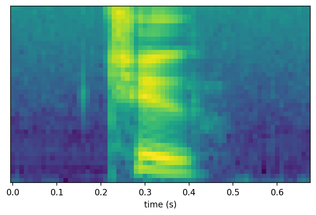
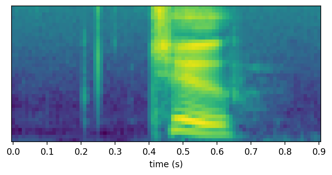
One great advantage of representing speech as spectrograms is that it enables us to visually analyze and classify speech segments. Below are two speech segments for the word two and one speech segment for the word one, spoken by the same speaker. We can tell that the segments in Figure 1 and 2 are visually similar and are quite different from the one in Figure 3. In this post, we will formalize this intuition.

Spectral Distortion
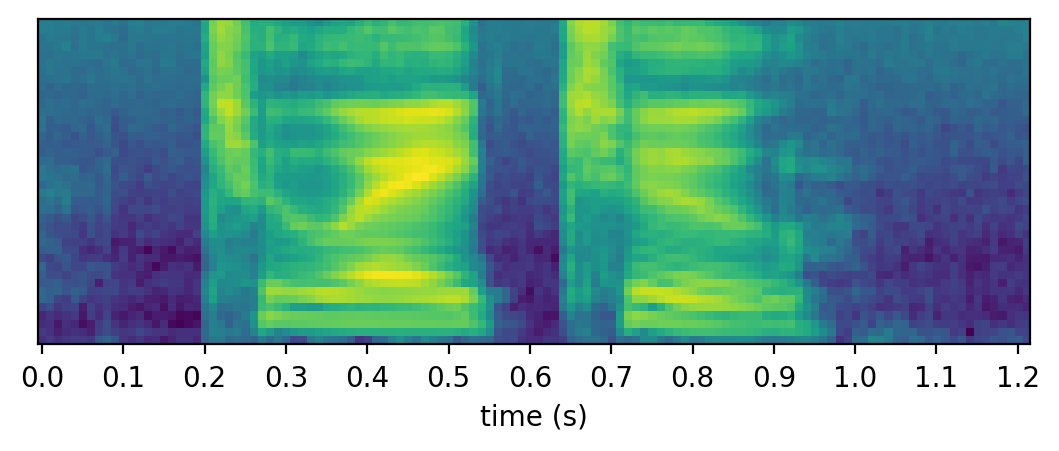
Recall that speech is nonstationary, meaning that its content changes over time. It we take a closer look at the speech segment in Figure 1, we can see several distinct regions, for example, the silence at the beginning and the end, the first phone [t], and the second phone [u]. To see the difference of these distinct regions, the same speech segment is shown in Figure 4 with more details. In particular, if we take slices of the spectrogram, often called spectra or frames, we can see that at time 0.1s, 0.25s, and 0.35s (shown in Figure 4) are significantly different from each other.

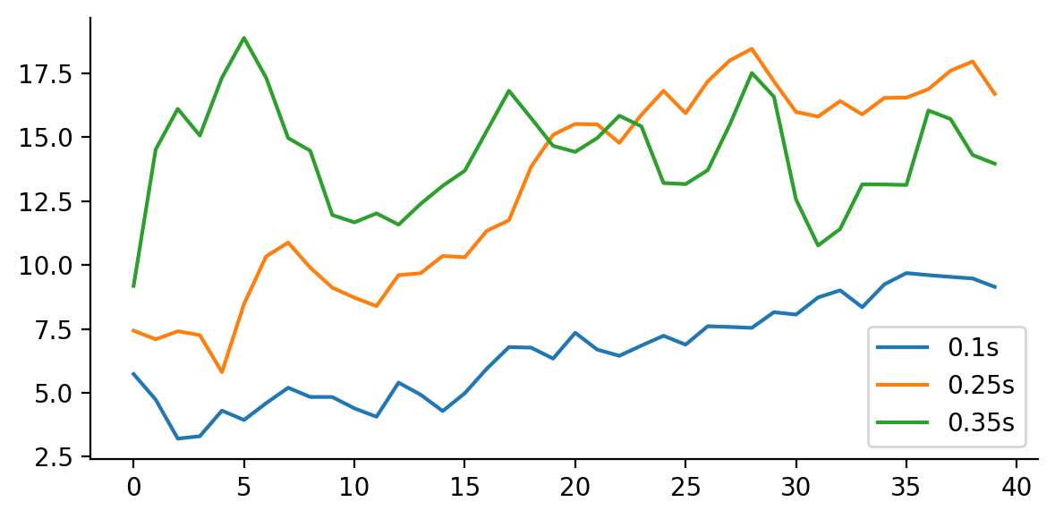
The problem of measuring the similarity of speech segments inevitably involves measuring the similarity of frames. In this post, we simply use the $\ell_2$ norm as the distance of two spectra. More formally, we represent a frame as a vector, in our case, a 40-dimensional vector. The distance between two frames $x$ and $y$ is measured by \begin{align} \|x - y\|_2 = \sqrt{\sum_{i=1}^d (x_i - y_i)^2}. \end{align} There are many other alternatives, and the family of distances is generally called spectral-distortion measures. We will stick to $\ell_2$ for the rest of the post, but it is easy to plug and play different distance functions into the formulation we are going to discuss.
Given two speech segments, one of $T_1$ frames and the other of $T_2$ frames, there are only $T_1 T_2$ distances to consider. The distances can be represented as a matrix, and is shown in Figure 6 along with the speech segments. We can see a dark diagonal line around the center of the distance matrix. The dark line shows us a path to go from the bottom left to the top right while incurring the lowest distortion. In other words, the dark line tells us how the frames in the two speech segments should be matched or aligned.

Since no two words, even for the same speaker, can be pronounced exactly the same way, we have to account for certain variance when comparing two speech segments. One hypothesis is that the words being uttered remain the same to a listener, as long as certain targets are met as the speaker produces the speech. As a consequence, we should be able to align two speech segments if they contain the same set of targets.
The approach we are going to discuss lets the spectral-distortion measures to handle spectral variance, and lets the alignment handle the variance of speaking rate. This approach assumes that spectral changes are completely synchronized in time. This is of course idealized, but we can go really far with this simple idea.
Dynamic Time Warping (DTW)
There are two constraints to consider when aligning two speech segments.
- Every frame needs to be aligned.
- When a frame is aligned to a frame at a particular time, subsequent frames can only be aligned to frames no earlier than that time.
The problem of finding the alignment of minimum distortion can be decomposed into sub-problems. In particular, we can ask the question: Does knowing the result of aligning $X_{1:s-1}$ to $Y_{1:t}$ and similar cases makes it simpler to align $X_{1:s}$ and $Y_{1:t}$? Indeed, we only need to consider how to align $X_s$ if we know how to align $X_{1:s-1}$ and $Y_{1:t}$. In general, we have the recursion \begin{align} d[s, t] = \min \Bigg\{ d[s, t-1], d[s-1, t], d[s-1, t-1] \Bigg\} + \|X_{s} - Y_{t}\|. \end{align} In words, to align $X_{1:s}$ and $Y_{1:t}$, we can first align $X_{1:s-1}$ with $Y_{1:t}$, align $X_{1:s}$ with $Y_{1:t-1}$, align $X_{1:s-1}$ with $Y_{1:t-1}$, and align the final frames to find the minimum distortion.
The algorithm above is called dynamic time warping, and is based on classical dynamic programming. Other variants exist, for example, allowing frames to be discarded instead of aligned. The alignment of minimum distortion is shown in Figure 7 as a red line.

Note that the alignment is off diagonal at the beginning. It's because the silence frames look more or less the same, and it does not matter much how we align them. To avoid this unnecessary problem, we can excise the silence. The alignment is shown in Figure 8.

Template Matching
In addition to obtaining an alignment between speech segments, the minimum distortion can serve as a distance measure between speech segments. Table 1 shows the minimum distortions of the excised two against the other speech segments. It is clear that the distortions are lower when the word are the same than when the words are different. In other words, we can use distortions to identify the existence of a word. We refer to the word spectrograms without silence as templates. To recognize speech, a naive approach is to run an utterance through DTW against a library of templates. The sequence of word templates that has the lowest distortion would be the potential spoken words in the utterance.
| Two (Figure 1) | Two (Figure 2) | One (Figure 3) | |
| Two (without silence) | 379.10 | 585.71 | 917.95 |
To illustrate this idea, we can consider the speech in Figure 9. It consists of three words two eight two. To recognize the words, we can run DTW against various combination of templates. The alignment of Figure 9 with the concatenation of the templates two eight two is shown in Figure 10.

We obviously do not want to run DTW on combinatorially many word sequences. We again leverage dynamic programming to turn this into a tractable problem. The key observation is that it is relatively cheap to compute DTW against a sequence of word templates as long as the DTW of the prefix of the templates has been computed. In other words, we can keep the DTW traces, and keep concatenating word templates to match longer word sequences. when we decide to concatenate a word template onto a sequence of templates that is already been matched, we can simply continue the dynamic programming by extending the table with more entries. The decision left is what word template to choose for concatenation.
We can organize the decisions of what word template to use as a graph (shown in Figure 11). There are two benefits of representing the decisions of word templates as a graph. First, it is now clear what computation of dynamic programming can be reused. More importantly, we can now see template matching as a graph search problem, where the weights on the graph are the minimum distortion computed by DTW.
