A*
a posteriori probability
a priori probability
aberration
absolute conic
absolute coordinates
absolute orientation
absolute point
absolute quadric
absorption
accumulation method
accumulative difference
accuracy
acoustic sonar
ACRONYM
active appearance model
active blob
active contour model
active contour tracking
active illumination
active learning
active net
active sensing
active shape model
active stereo
active surface
active triangulation
active vision
active volume
activity analysis
acuity
adaptive
adaptive coding
adaptive contrast enhancement
adaptive edge detection
adaptive filtering
adaptive histogram equalization
adaptive Hough transform
adaptive meshing
adaptive pyramid
adaptive reconstruction
adaptive smoothing
adaptive thresholding
adaptive triangulation
adaptive visual servoing
additive color
additive noise
adjacency
adjacency graph
adjacent
affine
affine arc length
affine camera
affine curvature
affine flow
affine fundamental matrix
affine invariant
affine invariant region
affine length
affine moment
affine quadrifocal tensor
affine reconstruction
affine stereo
affine transformation
affine trifocal tensor
agglomerative clustering
albedo
algebraic distance
aliasing
alignment
ALVINN
ambient light
AMBLER
amplifier noise
analytic curve finding
anamorphic lens
anatomical map
AND operator
angiography
angularity ratio
anisotropic filtering
anomalous behavior detection
antimode
aperture
aperture control
aperture problem
apparent contour
apparent motion
appearance
appearance based recognition
appearance based tracking
appearance change
appearance enhancement
appearance flow
appearance model
appearance prediction
appearance singularity
arc length
arc of graph
architectural model reconstruction
area
area based
array processor
arterial tree segmentation
articulated object
articulated object model
articulated object segmentation
articulated object tracking
aspect
aspect graph
aspect ratio
association graph
astigmatism
atlas registration
atlas-based segmentation
ATR
attention
attentuation
attributed graph
augmented reality
autocalibration
autocorrelation
autofocus
automatic
automatic target recognition
autonomous vehicle
autoregressive model
autostereoscopic
average smoothing
AVI
axial representation
axis of elongation
axis of rotation
axis-angle curve representation
A*: A search technique that performs best-first searching based on an evaluation function that combines the cost so far and the estimated cost to the goal.
a posteriori probability: Literally, "after" probability. It is the probability
a priori probability: Suppose that there is a set Q of equally likely outcomes for a given action. If a particular event E could occur of any one of a subset S of these outcomes, then the a priori or theoretical probability of E is defined by

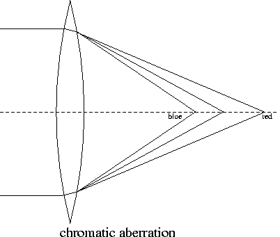
aberration: Problem exhibited by a lens or a mirror whereby unexpected results are obtained. There are two types of aberration commonly encountered: chromatic aberration, where different frequencies of light focus at different positions,
 |
absolute conic: The conic in 3D projective space that is the intersection of the unit (or any) sphere with the plane at infinity. It consists only of complex points. Its importance in computer vision is due to its role in the problem of autocalibration : the image of the absolute conic (IAC), a 2D conic, is represented by a
absolute coordinates: Generally used in contrast to local or relative coordinates. A coordinate system that is referenced to some external datum. For example, a pixel in a satellite image might be at (100,200) in image coordinates, but at (51:48:05N, 8:17:54W) in georeferenced absolute coordinates.
absolute orientation: In photogrammetry, the problem of registering two corresponding sets of 3D points. Used to register a photogrammetric reconstruction to some absolute coordinate system. Often expressed as the problem of determining the rotation

absolute point: A 3D point defining the origin of a coordinate system.
absolute quadric: The symmetric
 . Like the
absolute conic
, it is defined to be invariant under Euclidean transformations, is rescaled under similarities, takes the form
 under affine transforms and becomes an arbitrary
absorption: Attenuation of light caused by passing through an optical system or being incident on an object surface.
accumulation method: A method of accumulating evidence in histogram form, then searching for peaks, which correspond to hypotheses. See also Hough transform , generalized Hough transform .
accumulative difference: A means of detecting motion in image sequences. Each frame in the sequence is compared to a reference frame (after registration if necessary) to produce a difference image. Thresholding the difference image gives a binary motion mask. A counter for each pixel location in the accumulative image is incremented every time the difference between the reference image and the current image exceeds some threshold. Used for change detection .
accuracy: The error of a value away from the true value. Contrast this with precision .
acoustic sonar: SOund Navigation And Ranging. A device that is used primarily for the detection and location of objects (e.g., underwater or in air, as in mobile robotics, or internal to a human body, as in medical ultrasound ) by reflecting and intercepting acoustic waves. It operates with acoustic waves in an analogous way to that of radar , using both the time of flight and Doppler effects, giving the radial component of relative position and velocity.
ACRONYM: A vision system developed by Brooks that attempted to recognize three dimensional objects from two dimensional images, using generalized cylinder primitives to represent both stored model and objects extracted from the image.
active appearance model: A generalization of the widely used active shape model approach that includes all of the information in the image region covered by the target object, rather than just that near modeled edges. The active appearance model has a statistical model of the shape and gray-level appearance of the object of interest. This statistical model generalizes to cover most valid examples. Matching to an image involves finding model parameters that minimize the difference between the image and a synthesized model example, projected into the image.
active blob: A region based approach to the tracking of non-rigid motion in which an active shape model is used. The model is based on an initial region that is divided using Delaunay triangulation and then each patch is tracked from frame to frame (note that the patches can deform).
active contour models: A technique used in model based vision where object boundaries are detected using a deformable curve representation such as a snake . The term active refers to the ability of the snake to deform shape to better match the image data. See also active shape model .
active contour tracking: A technique used in model based vision where object boundaries are tracked in a video sequence using active contour models .
active illumination: A system of lighting where intensity, orientation, or pattern may be continuously controlled and altered. This kind of system may be used to generate structured light .
active learning: Learning about the environment through interaction (e.g., looking at an object from a new viewpoint).
active net: An active shape model that parameterizes a triangulated mesh.
active sensing: 1) A sensing activity carried out in an active or purposive way, for instance where a camera is moved in space to acquire multiple or optimal views of an object. (See also active vision , purposive vision , sensor planning .) 2) A sensing activity implying the projection of a pattern of energy, for instance a laser line, onto the scene. See also laser stripe triangulation , structured light triangulation .
active shape model: Statistical models of the shapes of objects that can deform to fit to a new example of the object. The shapes are constrained by a statistical shape model so that they may vary only in ways seen in a training set. The models are usually formed by using principal component analysis to identify the dominant modes of shape variation in observed examples of the shape. Model shapes are formed by linear combinations of the dominant modes.
active stereo: An alternative approach to traditional binocular stereo . One of the cameras is replaced with a structured light projector, which projects light onto the object of interest. If the camera calibration is known, the triangulation for computing the 3D coordinates of object points simply involves finding the intersection of a ray and known structures in the light field.
active surface: 1) A surface determined using a range sensor ; 2) an active shape model that deforms to fit a surface.
active triangulation: Determination of surface depth by triangulation between a light source at a known position and a camera that observes the effects of the illuminant on the scene. Light stripe ranging is one form of active triangulation. A variant is to use a single scanning laser beam to illuminate the scene and use a stereo pair of cameras to compute depth.
active vision: An approach to computer vision in which the camera or sensor is moved in a controlled manner, so as to simplify the nature of a problem. For example, rotating a camera with constant angular velocity while maintaining fixation at a point allows absolute calculation of scene point depth, instead of only relative depth that depends on the camera speed. (See also kinetic depth .)
active volume: The volume of interest in a machine vision application.
activity analysis: Analyzing the behavior of people or objects in a video sequence, for the purpose of identifying the immediate actions occurring or the long term sequence of actions. For example, detecting potential intruders in a restricted area.
acuity: The ability of a vision system to discriminate (or resolve) between closely arranged visual stimuli. This can be measure using a grating, i.e., a pattern of parallel black and white stripes of equal widths. Once the bars become too close, the grating becomes indistinguishable from a uniform image of the same average intensity as the bars. Under optimal lighting, the minimum spacing that a person can resolve is 0.5 min of arc.
adaptive: The property of an algorithm to adjust its parameters to the data at hand in order to optimize performance. Examples include adaptive contrast enhancement , adaptive filtering and adaptive smoothing .
adaptive coding: A scheme for the transmission of signals over unreliable channels, for example a wireless link. Adaptive coding varies the parameters of the encoding to respond to changes in the channel, for example "fading", where the signal-to-noise ratio degrades.
adaptive contrast enhancement: An image processing operation that applies histogram equalization locally across an image.
adaptive edge detection: Edge detection with adaptive thresholding of the gradient magnitude image.
adaptive filtering: In signal processing, any filtering process in which the parameters of the filter change over time, or where the parameters are different at different parts of the signal or image.
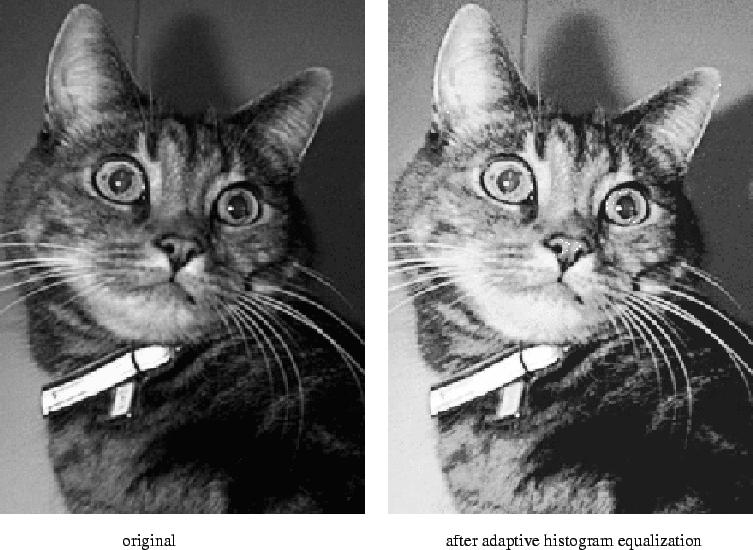
adaptive histogram equalization: A localized method of improving image contrast. A histogram is constructed of the gray levels present. These gray levels are re-mapped so that the histogram is approximately flat. It can be made perfectly flat by dithering.
 |
adaptive Hough transform: A Hough transform method that iteratively increases the resolution of the parameter space quantization. It is particularly useful for dealing with high dimensional parameter spaces. Its disadvantage is that sharp peaks in the histogram can be missed.
adaptive meshing: Methods for creating simplified meshes where elements are made smaller in regions of high detail (rapid changes in surface orientation) and larger in regions of low detail, such as planes.
adaptive pyramid: A method of multi-scale processing where small areas of image having some feature in common (say color) are first extracted into a graph representation. This graph is then manipulated, for example by pruning or merging, until the level of desired scale is reached.
adaptive reconstruction: Data driven methods for creating statistically significant data in areas of a 3D data cloud where data may be missing due to sampling problems.
adaptive smoothing: An iterative smoothing algorithm that avoids smoothing over edges. Given an image
- Compute gradient magnitude image

- Make weights image

- Smooth the image
where


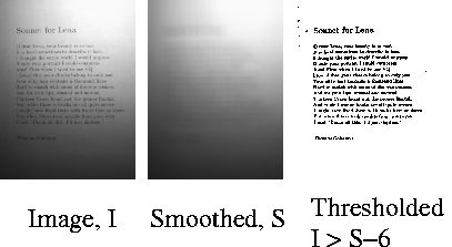
adaptive thresholding: An improved image thresholding technique where the threshold value is varied at each pixel. A common technique is to use the average intensity in a neighbourhood to set the threshold.
 |
adaptive triangulation: See adaptive meshing .
adaptive visual servoing: See visual servoing.
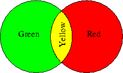
additive color: The way in which multiple wavelengths of light can be combined to allow other colors to be perceived (e.g., if equal amounts of green and red light are shone on a sheet of white paper the paper will appear to be illuminated with a yellow light source. Contrast this with subtractive color .
 |
additive noise: Generally image independent noise that is added to it by some external process. The recorded image
adjacent: Commonly meaning "next to each other", whether in a physical sense of being connected pixels in an image, image regions sharing some common boundary, nodes in a graph connected by an arc or components in a geometric model sharing some common bounding component, etc. Formally defining "adjacent" can be somewhat heuristic because you may need a way to specify closeness (e.g., on a quantized grid of pixels) or consider how much shared "boundary" is required before two structures are adjacent.
adjacency: See adjacent.
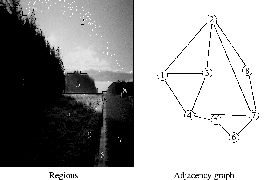
adjacency graph: A graph that shows the adjacency between structures, such as segmented image regions . The nodes of the graph are the structures and an arc implies adjacency of the two structures connected by the arc. This figure shows the graph associated with the segmented image on the left:
 |
affine: A term first used by Euler. Affine geometry is a study of properties of geometric objects that remain invariant under affine transformations (mappings). These include: parallelness, cross ratio, adjacency.
affine arc length: For a parametric equation of a curve

affine camera: A special case of the projective camera that is obtained by constraining the
affine curvature: A measure of curvature based on the affine arc length ,
affine flow: A method of finding the movement of a surface patch by estimating the affine transformation parameters required to transform the patch from its position in one view to another.
affine fundamental matrix: The fundamental matrix which is obtained from a pair of cameras under affine viewing conditions. It is a
affine invariant: An object or shape property that is not changed (i.e., is invariant) by the application of an affine transformation . See also invariant.
affine invariant region: Image patches that automatically deform with changing viewpoint in such a way that they cover identical physical parts of a scene. Since such regions can are describable by a set of invariant features they are relatively easy to match between views under changing illumination .
affine length: See affine arc length .
affine moment: Four shape measures derived from second- and third-order moments that remain invariant under affine transformation s. They are given by:

|
| |||
|
|
|||
where each
affine quadrifocal tensor: The form taken by the quadrifocal tensor when specialized to the viewing conditions modeled by the affine camera .
affine reconstruction: A three dimensional reconstruction where the ambiguity in the choice of basis is affine only. Planes that are parallel in the Euclidean basis are parallel in the affine reconstruction. A projective reconstruction can be upgraded to affine by identification of the plane at infinity, often by locating the absolute conic in the reconstruction.
affine stereo: A method of scene reconstruction using two calibrated views of a scene from known view points. It is a simple but very robust approximation to the geometry of stereo vision, to estimate positions, shapes and surface orientations. It can be calibrated very easily by observing just four reference points. Any two views of the same planar surface will be related by an affine transformation that maps one image to the other. This consists of a translation and a tensor, known as the disparity gradient tensor representing the distortion in image shape. If the standard unit vectors X and Y in one image are the projections of some vectors on the object surface and the linear mapping between images is represented by a
affine transformation: A special set of transformations in Euclidean geometry that preserve some properties of the construct being transformed.
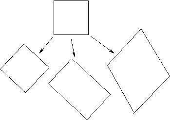 |
- Collinearity of points: if three points belong to the same straight line, their images under affine transformations also belong to the same line and the middle point remains between the other two points.
- Parallel lines remain parallel, concurrent lines remain concurrent (images of intersecting lines intersect).
- The ratio of length of line segments of a given line remains constant.
- The ratio of areas of two triangles remains constant.
- Ellipses remain ellipses and the same is true for parabolas and hyperbolas.
- Barycenters of triangles (and other shapes) map into the corresponding barycenters.
affine trifocal tensor: The form taken by the trifocal tensor when specialized to the viewing conditions modeled by the affine camera .
agglomerative clustering: A class of iterative clustering algorithms that begin with a large number of clusters and at each iteration merge pairs (or tuples) of clusters. Stopping the process at a certain number of iterations gives the final set of clusters, or the process can be run until only one cluster remains, and the progress of the algorithm represented as a dendrogram.
albedo: Whiteness. Originally a term used in astronomy to describe reflecting power.
 |
algebraic distance: A linear distance metric commonly used in computer vision applications because of its simple form and standard matrix based least mean square estimation operations. If a curve or surface is defined implicitly by
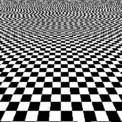
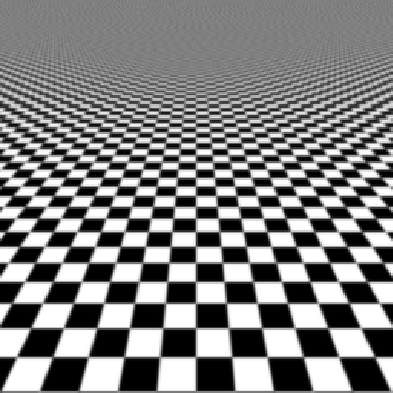
aliasing: The erroneous replacement of high spatial frequency (HF) components by low-frequency ones when a signal is sampled . The affected HF components are those that are higher than the Nyquist frequency, or half the sampling frequency. Examples include the slowing of periodic signals by strobe lighting, and corruption of areas of detail in image resizing. If the source signal has no HF components, the effects of aliasing are avoided, so the low pass filtering of a signal to remove HF components prior to sampling is one form of anti-aliasing. The image below is the perspective projection of a checkerboard. The image is obtained by sampling the scene at a set of integer locations. First figure: The spatial frequency increases as the plane recedes, producing aliasing artifacts (jagged lines in the foreground, moiré patterns in the background). Second figure: removing high-frequency components (i.e., smoothing ) before downsampling mitigates the effect.
 |
 |
alignment: An approach to geometric model matching by registering a geometric model to the image data.
ALVINN: Autonomous Land Vehicle In a Neural Network. An early attempt, at Carnegie-Mellon University, to learn a complex behaviour (maneuvering a vehicle) by observing humans.
ambient light: Illumination by diffuse reflections from all surfaces within a scene (including the sky, which acts as an external distant surface). In other words, light that comes from all directions, such as the sky on a cloudy day. Ambient light ensures that all surfaces are illuminated, including those not directly facing light sources.
AMBLER: An autonomous active vision system using both structured light and sonar, developed by NASA and Carnegie-Mellon University. It is supported by a 12-legged robot and is intended for planetary exploration.
amplifier noise: Spurious additive noise signal generated by the electronics in a sampling device. The standard model for this type of noise is Gaussian. It is independent of the signal. In color cameras, where more amplification is used in the blue color channel than in the green or red channel there tends to be more noise in the blue channel. In well-designed electronics amplifier noise is generally negligible.
analytic curve finding: A method of detecting parametric curves by first transforming data into a feature space that is then searched for the hypothesized curve parameters. Examples might be line finding using the Hough transform .
anamorphic lens: A lens having one or more cylindrical surfaces. Anamorphic lenses are used in photography to produce images that are compressed in one dimension. Images can later be restored to true form using another reversing anamorphic lens set. This form of lens is used in wide-screen movie photography.
anatomical map: A biological model usable for alignment with or region labeling of a corresponding image dataset. For example, one could use a model of the brain's functional regions to assist in the identification of brain structures in an NMR dataset.
AND operator: A boolean logic operator that combines two input binary images, applying the AND logic
| 0 | 0 | 0 |
| 0 | 1 | 0 |
| 1 | 0 | 0 |
| 1 | 1 | 1 |
at each pair of corresponding pixels. This approach is used to select image regions. The rightmost image below is the result of ANDing the two leftmost images.
 |
angiography: A method for imaging blood vessels by introducing a dye that is opaque when photographed by X-ray. Also the study of images obtained in this way.
angularity ratio: Given two figures,


anisotropic filtering: Any filtering technique where the filter parameters vary over the image or signal being filtered.
anomalous behavior detection: Special case of surveillance where human movement is analyzed. Used in particular to detect intruders or behavior likely to precede or indicate crime.
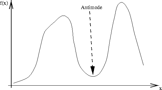
antimode: The minimum between two maxima. For example one method of threshold selection is done by determining the antimode in a bimodal histogram.
 |
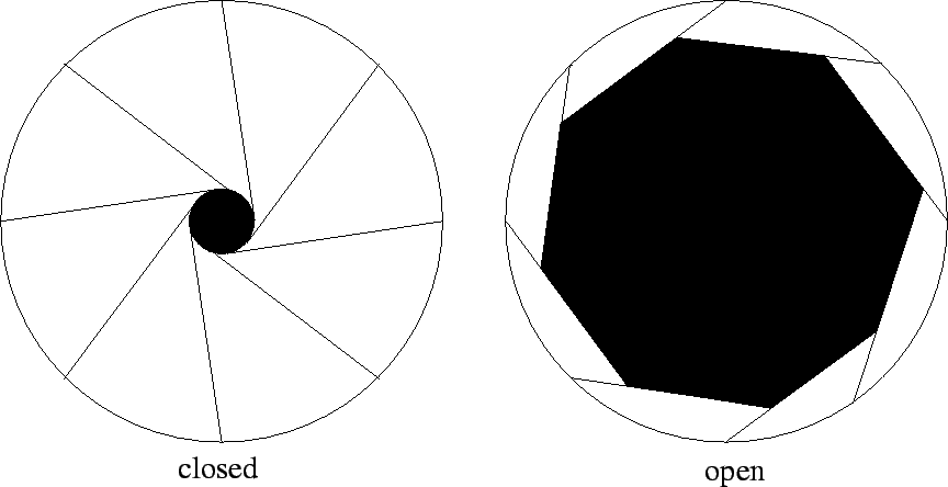
aperture: Opening in the lens diaphragm of a camera through which light is admitted. This device is often arranged so that the amount of light can be controlled accurately. A small aperture reduces the amount of light available, but increases the depth of field . This figure shows nearly closed (left) and nearly open (right) aperture positions:
 |
aperture control: Mechanism for varying the size of a camera's aperture .
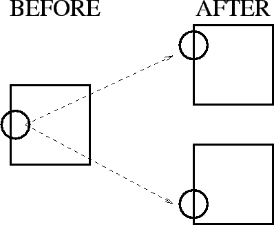
aperture problem: If a motion sensor has a finite receptive field, it perceives the world through something resembling an aperture, making the motion of a homogeneous contour seem locally ambiguous. Within that aperture, different physical motions are therefore indistinguishable. For example, the two alternative motions of the square below are identical in the circled receptive fields:
 |
apparent contour: The apparent contour of a surface
apparent motion: The 3D motion suggested by the image motion field , but not necessarily matching the real 3D motion. The reason for this mismatch is the motion fields may be ambiguous, that is, may be generated by different 3D motions, or light source movement. Mathematically, there may be multiple solutions to the problem of reconstructing 3D motion from the image motion field. See also visual illusion , motion estimation .
appearance: The way an object looks from a particular viewpoint under particular lighting conditions.
appearance based recognition: Object recognition where the object model encodes the possible appearances of the object (as contrasted with a geometric model that encodes the shape as used in model based recognition ). In principle, it is impossible to encode all appearances when occlusions are considered; however, small numbers of appearances can often be adequate, especially if there are not many models in the model base. There are many approaches to appearance based recognition, such as using a principal component model to encode all appearances in a compressed framework, using color histograms to summarize the appearance, or using a set of local appearance descriptors such as Gabor filters extracted at interest points . A common feature of these approaches is learning the models from examples.
appearance based tracking: Methods for object or target recognition in real time, based on image pixel values in each frame rather than derived features. Temporal filtering, such as the Kalman filter , is often used.
appearance change: Changes in an image that are not easily accounted for by motion, such as an object actually changing form.
appearance enhancement transform: Generic term for operations applied to images to change, or enhance, some aspect of them. Examples include brightness adjustment, contrast adjustment, edge sharpening, histogram equalization, saturation adjustment or magnification.
appearance flow: Robust methods for real time object recognition from a sequence of images depicting a moving object. Changes in the images are used rather than the images themselves. It is analogous to processing using optical flow .
appearance model: A representation used for interpreting images that is based on the appearance of the object. These models are usually learned by using multiple views of the objects. See also active appearance model and appearance based recognition .
appearance prediction: Part of the science of appearance engineering, where an object texture is changed so that the viewer experience is predictable.
appearance singularity: An image position where a small change in viewer position can cause a dramatic change in the appearance of the observed scene, such as the appearance or disappearance of image features. This is contrasted with changes occurring when in a generic viewpoint . For example, when viewing the corner of a cube from a distance, a small change in viewpoint still leaves the three surfaces at the corner visible. However, when the viewpoint moves into the infinite plane containing one of the cube faces (a singularity), one or more of the planes disappears.
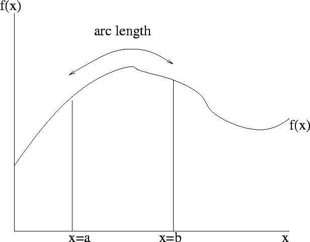
arc length: If
![$\displaystyle \int_a^b \sqrt{1+[f'(x)]^2}dx $](CVFIG5/img110.png)
 |
arc of graph: Two nodes in a graph can be connected by an arc. The dashed lines here are the arcs:
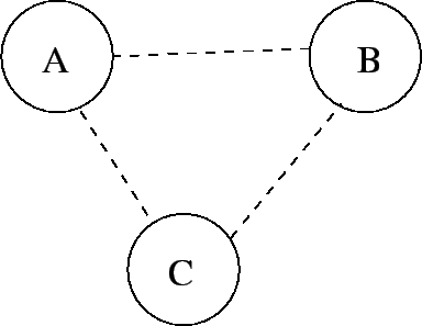 |
architectural model reconstruction: A generic term for reverse engineering buildings based on collected 3D data as well as libraries of building constraints.
area: The measure of a region or surface's extension in some given units. The units could be image units, such as square pixels, or in scene units, such as square centimeters.
area based: Image operation that is applied to a region of an image, as opposed to pixel based.
array processor: A group of time-synchronized processing elements that perform computations on data distributed across them. Some array processors have elements that communicate only with their immediate neighbors, as in the topology shown below. See also single instruction multiple data .
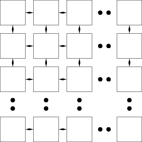 |
arterial tree segmentation: Generic term for methods used in finding internal pipe-like structures in medical images. Example image types are NMR images, angiograms and X-rays . Example trees are bronchial systems and veins.
articulated object: An object composed by a number of (usually) rigid subparts or components connected by joints, which can be arranged in a number of different configurations. The human body is a typical example.
articulated object model: A representation of an articulated object that includes both its separate parts and their range of movement (typically joint angles) relative to each other.
articulated object segmentation: Methods for acquiring an articulated object from 2D or 3D data.
articulated object tracking: Tracking an articulated object in an image sequence. This includes both the pose of the object and also its shape parameters, such as joint angles.
aspect graph: A graph of the set of views (aspects) of an object, where the arcs of the graph are transitions between two neighboring views (the nodes ) and a change between aspects is called a visual event. See also characteristic view . This graph shows some of the aspects of the hippopotamus
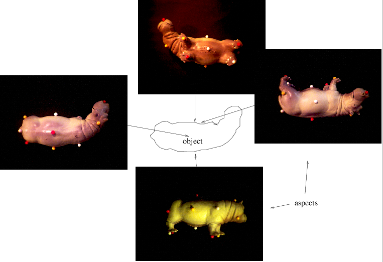 |
aspect ratio: 1) The ratio of the sides of the bounding box of an object, where the orientation of the box is chosen to maximize this ratio. Since this measure is scale invariant it is a useful metric for object recognition . 2) In a camera, it is the ratio of the horizontal to vertical pixel sizes. 3) In an image, it is the ratio of the image width to height. For example, an image of 640 by 480 pixels has an aspect ratio of 4:3.
aspects: See characteristic view and aspect graph .
association graph: A graph used in structure matching, such as matching a geometric model to a data description. In this graph, each node corresponds to a pairing between a model and a data feature (with the implicit assumption that they are compatible). Arcs in the graph mean that the two connected nodes are pairwise compatible. Finding maximal cliques is one technique for finding good matches. The graph below shows a set of pairings of model features A, B and C with image features a, b, c and d. The maximal clique consisting of A:a, B:b and C:c is one match hypothesis.
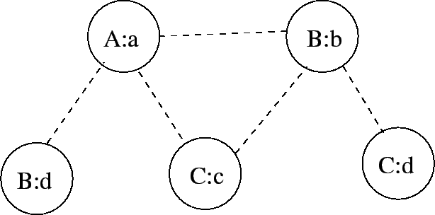 |
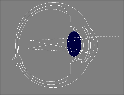
astigmatism: Astigmatism is a refractive error where the light is focused within an optical system, such as in this example.
 |
atlas based segmentation: A segmentation technique used in medical image processing, especially with brain images. Automatic tissue segmentation is achieved using a model of the brain structure and imagery (see atlas registration ) compiled with the assistance of human experts. See also image segmentation .
atlas registration: An image registration technique used in medical image processing, especially to register brain images. An atlas is a model (perhaps statistical) of the characteristics of multiple brains, providing examples of normal and pathological structures. This makes it possible to take into account anomalies that single-image registration could not. See also medical image registration .
ATR: See automatic target recognition .
attention: See visual attention .
attenuation: The reduction of a particular phenomenon, for instance, noise attenuation as the reduction of image noise.
attributed graph: A graph useful for representing different properties of an image. Its nodes are attributed pairs of image segments, their color or shape for example. The relations between them, such as relative texture or brightness are encoded as arcs .
augmented reality: Primarily a projection method that adds graphics or sound, etc as an overlay to original image or audio. For example, a fire-fighter's helmet display could show exit routes registered to his/her view of the building.
autocalibration: The recovery of a camera's calibration using only point (or other feature) correspondences from multiple uncalibrated images and geometric consistency constraints (e.g., that the camera settings are the same for all images in a sequence).
autocorrelation: The extent to which a signal is similar to shifted copies of itself. For an infinitely long 1D signal


autofocus: Automatic determination and control of image sharpness in an optical or vision system. There are two major variations in this control system: active focusing and passive focusing. Active autofocus is performed using sonar or infrared signal to determine the object distance. Passive autofocus is performed by analyzing the image itself to optimize differences between adjacent pixels in the CCD array.
automatic: Performed by a machine without human intervention. The opposite of "manual".
automatic target recognition (ATR): Sensors and algorithms used for detecting hostile objects in a scene. Sensors are of many different types, sampling in infrared , visible light and using sonar and radar .
autonomous vehicle: A mobile robot controlled by computer, with human input operating only at a very high level, stating the ultimate destination or task for example. Autonomous navigation requires the visual tasks of route detection, self-localization , landmark location and obstacle detection , as well as robotics tasks such as route planning and motor control.
autoregressive model: A model that uses statistical properties of past behavior of some variable to predict future behavior of that variable. A signal
autostereogram: An image similar to a random dot stereogram in which the corresponding features are combined into a single image. Stereo fusion allows the perception of a 3D shape in the 2D image.
average smoothing: See mean smoothing .
AVI: Microsoft format for audio and video files ("audio video interleaved"). Unlike MPEG, it is not a standard, so that compatibility of AVI video files and AVI players is not always guaranteed.
axial representation: A region representation that uses a curve to describe the image region. The axis may be a skeleton derived from the region by a thinning process.
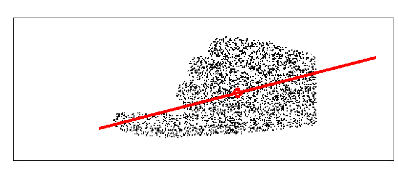
axis of elongation: 1) The line that minimizes the second moment of the data points. If
 |
axis of rotation: A line about which a rotation is performed. Equivalently, the line whose points are fixed under the action of a rotation. Given a 3D rotation matrix
axis-angle curve representation: A rotation representation based on the amount of twist