Catadioptric Projection Geometry

Martin King 0454718

Catadioptric projection systems are systems which employ both reflective optics (catoptrics) and refractive optics (dioptric). This means that images are produced through the use of both mirrors and lenses.

(image taken from [1] Geyer C, Daniilidis)

These systems can be split into two groups, the central projection systems and the non-central projection systems.

Central Projection Systems

A central projection system is perhaps the more commonly used, and is a system which has a single effective viewpoint. These systems can include the use of planar, elliptical, parabolic or hyperbolic mirrors.

This is normally the most desired form of catadioptric system as it removes the issue of parallax in projecting the geometry onto a plane.

Non-Central Projection Systems

Non-central projection systems do not use a single viewpoint and instead use a locus of different viewpoints, called a caustic. Such systems can use spherical or conical mirrors and can have an advantage of having a wider field of view and a higher image resolution.

Also, it is always possible to have a misalignment in a central projection system that can result in a non-single viewpoint as well.

However, due to the complex nature of the non-single viewpoint systems, only the geometry of the central projection will be given

Central Projection Geometry

Geyer and Daniilidis [1] have created a unifying theory for central projection catadioptric systems. For central projection systems, whose mirrors have conic cross-sections, the geometry can be simplified to a central projection to a sphere centered about the viewpoint, followed by central projection from a point on the sphere’s axis.

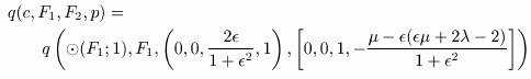
The 3D catadioptric projection is defined as the quadratic map

q(c, F₁, F₂, p)

Where c is a conic with foci F₁ & F₂ rotated symmetrically around the z-axis, which can be considered as a sphere €(F₁;1) with centre F₁ and radius 1.

p is a plane (0, 0, 1, -μ), where μ is the y intercept of the plane.

F₁ has coordinates (0, 0, 0, 1)

F₂ has coordinates (0, 0, -2є, λ^-1(є²-1))

Where є is the eccentricity of the quadratic and λ is the scaling factor.

Which gives,

As this projection can be considered a spherical map, we define a spherical map, s_l,m as a quadratic projection

Where €(A;1) is a unit sphere centred on an arbitrary point A.

For elliptic projection (0 < є < 1)

F₁ = (0, 0, 0, 1), F₂ = (0, 0, 4pє, є²-1), p = (0, 0, 1, 0)

For parabolic projection (є = 1)

F₁ = (0, 0, 0, 1), F₂ = (0, 0, 1, 0), p = (0, 0, 1, 0)

For hyperbolic projection (є > 1)

F₁ = (0, 0, 0, 1), F₂ = (0, 0, 4pє, є²-1), p = (0, 0, 1, 0)

For each of these projections c is a conic of the projection type with foci F₁, F₂, and a latus rectum of 4p. Also, μ = 0 and λ = 2p

References & Useful Resources

[1] Geyer C, Daniilidis K, Catadioptric Projective Geometry, International Journal of Computer Vision 45(3), 223–243, 2001

http://www.cis.upenn.edu/~kostas/mypub.dir/geyer01ijcv.pdf

[2] Baker S, Nayar S K, A Theory of Catadioptric Image Formation, Proceedings in the 6^th International Conference of Computer Vision, 1998

http://citeseer.ist.psu.edu/baker98theory.html

[3] Barreto J P, Araujo H, Issues on the Geometry of Central Catadioptric Image Formation, Computer Vision and Pattern Recognition, 2001. CVPR 2001

[4] Swaminathan R, Grossberg MD, Nayar S K, Caustics of Catadioptric Cameras, Computer Vision, 2001. ICCV 2001, Proceedings Eighth

[5] Svoboda T, Pajdla T, Epipolar Geometry for Central Catadioptric Cameras, International Journal of Computer Vision 49(1), 23-27, 2002

http://iris.usc.edu/Vision-Notes/bibliography/compute70.html - a useful archive of catadioptric papers