


The concept of error covariance is very important in statistics
as it allows us to model linear correlations between parameters.
For locally linear fit functions f we can approximate the
variation in a  metric about the minimum value as a quadratic.
We will examine the two dimensional case first, for example:
metric about the minimum value as a quadratic.
We will examine the two dimensional case first, for example:

This can be written as

where  is defined as the inverse covariance matrix

Comparing with the above quadratic equation we get

where

Notice that the b and c coefficients are zero as required if the
 is at the minimum.
In the general case we need a method for determining the covariance
matrix for model fits with an arbitrary number of parameters.
Starting from the
is at the minimum.
In the general case we need a method for determining the covariance
matrix for model fits with an arbitrary number of parameters.
Starting from the  definition using the same notation as
previously.
definition using the same notation as
previously.

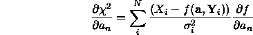
We can compute the first and second order derivatives as follows:
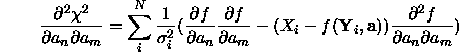
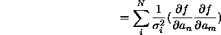
The second term in this equation is expected to be negligible compared to the first and with an expected value of zero if the model is a good fit. Thus the cross derivatives can be approximated to a good accuracy by
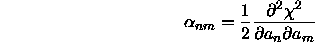
The following quantities are often defined.
As these derivatives must correspond to the first coefficients in
a polynomial (Taylor) expansion of the  function then,

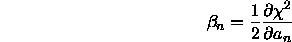
And the expected change in  for a small change in model
parameters can be written as
for a small change in model
parameters can be written as
