The Correspondences by Sensitivity to Movement (CSM) Algorithm
Elizabeth Guest, Leeds Metropolitan University
The CSM (correspondences by Sensitivity to Movement) algorithm is a robust method for calculating correspondences in both 2D and 3D images. The basic principle is to test the sensitivity of a possible correspondence to movement.
There are 3 stages to the CSM algorithm:
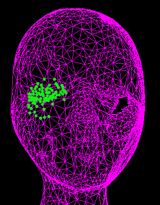
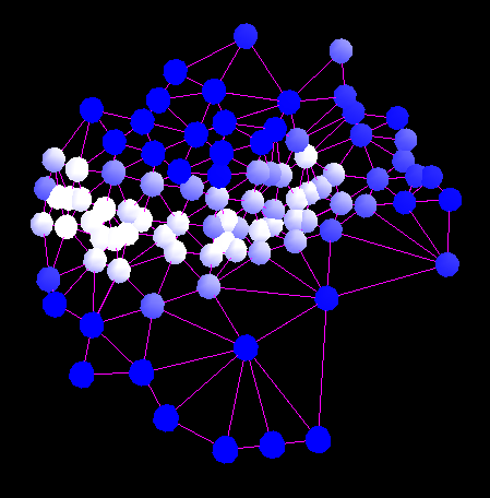
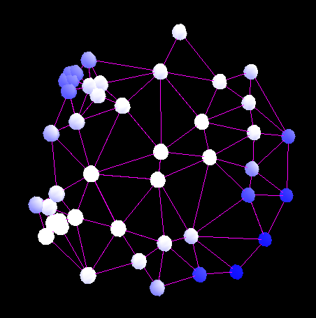
- Use an appropriate (see below) similarity measure to match a point (the matchpoint) of image A to points within a certain radius in image B. The points in image B, together with their similarity values to the matchpoint define a "matchmap". Note that if the two images are surfaces represented by a surface mesh, then a node of the surface mesh, representing image A, is matched to nodes of the surface mesh, representing image B.
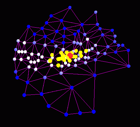
- Perform regular virtual movements of the matchpoint, and for each position of the matchpoint, calculate a "tentative corresponding point" on image B. Each tentative corresponding point is calculated by summing over the matchmap, while taking distances from the matchpoint to each point in the matchmap into account. Note that the tentative corresponding points are not constrained to coincide with one of the points in the matchmap and, in general, will lie between these points. The formula used to calculate each tentative corresponding point,
 , is:
, is:

where

for 2D images and

for 3D surface meshes. In these formulae,  is the vector from the matchpoint to point i in the matchmap; is the similarity value for point i, b is a constant; is the mean distance from node i in the surface mesh B to all the nodes connected to it; and
  is the number of nodes connected to node i. b is generally set to 2 so that that points that are far away can still influence the position of the corresponding point if they match well.
- Calculate a corresponding point and a measure of reliability by analyzing the distribution of the tentative corresponding points. If the tentative corresponding points are scattered along a line, the corresponding point is the closest point on the line to the matchpoint. Otherwise the centroid of the scatter of points is used. The eigenvalues obtained by a principal axes analysis of the scatter of points are used to determine whether the tentative corresponding points are scattered along a line or clustered around the point: if the first eigenvalue is significantly larger than the other eigenvalue(s), then the points are scattered along a line. The reliability is also derived from the eigenvalues:
 ,
, 
where t is the number of tentative corresponding points, d is the maximum displacement undergone by the matchpoint, and a is a variable between 0.0 and 1.0 which enables the reliability values to be tuned to the application. In the 2D and 3D surface cases, the second eigenvalue should be used as this is small both when the tentative corresponding points are scattered along a line and when they are scattered near a point. In the case of 3D volumes, the second eigenvalue should be chosen when the tentative corresponding points are scattered near a line; and the 3rd eigenvalue in all other cases.
The similarity measure
Note that in order for the correspondence calculations to work well, it is essential that the matchmap, and therefore the similarity measure satisfy the following criteria:
- There must be good discrimination between the good and bad matches. For best results the similarity measure should be tailored to the type of images in the application.
- The values generated by the similarity measure should be normalized to the range [0,1].
Examples of suitable similarity measures for 2D images and 3D surfaces are given below. Note that the 2D similarity measure, in particular, was designed for a specific application (serial histological sections), and may not be ideal for other applications.
2D similarity measure
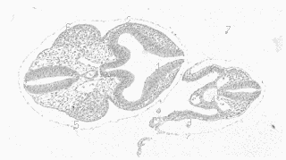
We give a suitable similarity measure for 2D serial sections of mouse embryos. In these images, different regions are characterized by the mean and standard deviation of their grey levels. Therefore, for these particular images, matching is based on the following features for each pixel:
- The direction of an edge segment centered on the pixel separating two regions.
- The strength of the edge. This is 1.0 when there is no edge at the pixel and greater than 1.0 when there is an edge.
- The means and standard deviations of the two regions separated by the edge segment.
This information is obtained for each pixel by passing a series of masks over the image. Each mask represents an edge direction and two regions, one on each side of the edge. A statistical test for small samples, the F-test, is used to compare the standard deviations of the pixels in the two regions in the mask and the mask giving the highest response to this test gives the edge direction and the two regions. This constitutes the F-test filter.
Points are matched from two images, A and B, by calculating a measure of similarity between pairs of corresponding regions. The corresponding regions of the two masks are given by the orientation of the line. In the following, the regions are denoted  ,
, and
and  ,
,  . The means of the grey values of the two regions can be compared with the T-test; and the variances can be compared with the F-test. By multiplying these quantities together, we obtain a function that varies depending on the similarities between the means and variances of two regions. In order to take account of both pairs of regions, the similarity measure used to compare the means and variances is
 ,
,
where and refer to the F- and T-tests applied to attributes from  and
and  . The values of this function are in the range [0,1], where 1 signifies that both pairs of regions have similar means and variances; and 0 signifies that these regions do not have similar means and variances. The parameters a and b were set to 1.0 and 2.0 respectively by an experiment designed to maximize the discrimination between good and bad matches.
The similarity measure must also include the difference in the directions of the edge segments centered on the two image points. This is done by means of the gaussian

The value of the parameter w should be chosen so that a small angle penalty is calculated for differences in angles up to the resolution of the line direction calculation (a value of 30 degrees was found to be suitable for 5 x 5 masks). The final similarity measure is:

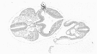
Matchpoints can be calculated by applying the F-filter to the image, thresholding the result to obtain the edges and thinning these edges using non-maximal suppression. Finally choose points from the resulting edges, starting with those with the highest values and making sure that all points are separated by a minimum distance.
2D example
3D similarity measure
Our 3D similarity measure is based on the normals and curvatures of the surfaces. Three quantities are compared:
- The curvedness defined as:

where  and
and  are the principal curvatures;

The shape is in the range [-1,1], where -1 denotes a spherical concave surface, and +1 a spherical convex surface.
- The relative angle, Q , between the normal and the vector from the main axis of symmetry of the object to a surface point. This is a new measure that helps to localize points in regions of uniform curvature. This works well as long as the surface does not resemble a cylinder. If the surface does resemble a cylinder then take the second vector from the centroid of the surface instead of the main axis of symmetry.
We define a separate measure for each of these quantities, and then multiply these measures together to give the matchvalue  , where l, h, and g are defined by:
Curvedness:

The factor 1000 is used to stop the values being swamped by 1.0, which has been included to prevent division by zero. Note that although the curvedness varies with scale, this match function is independent of scale.
Shape:

Relative angle:

We set the parameters  and
and  to 1/3 and p /18 respectively to allow for small differences in the surfaces and small errors in the calculation of S and Q .
3D example
Examples of the CSM algorithm applied to 2D images


matchpoints search regions
|

|

|

|
|
1 (1.00) |
2 (0.47) |
3 (0.96) |
|
|
|
|
|

|

|

|
|
4 (0.03) |
5 (0.25) |
6 (0.84) |
|
|
|
|
|

|

|

|
|
7 (0.10) |
8 (0.0) |
9 (0.05) |
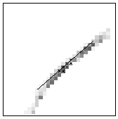
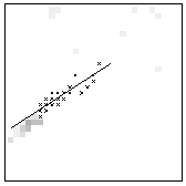
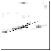
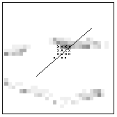
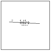
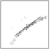
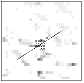
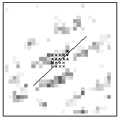
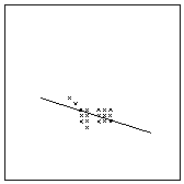
Matchmaps, tentative corresponding points (black crosses) and corresponding lines. The numbers in brackets are the reliability values.
back
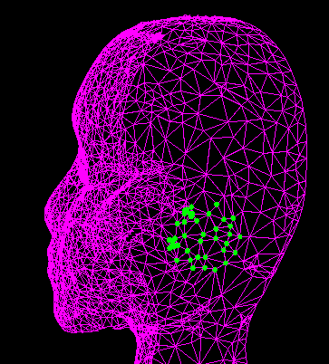
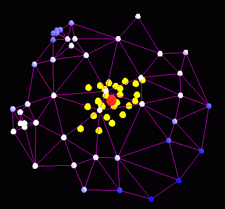
Examples of the CSM algorithm applied to facial surfaces
|

|

|
|
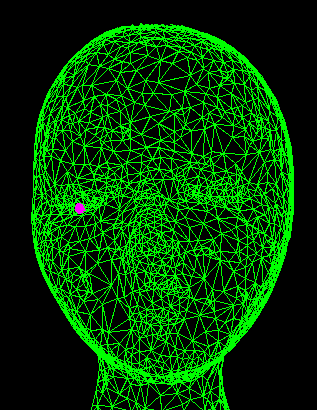
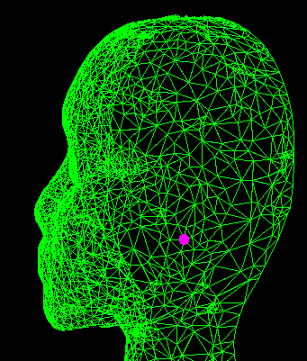
Matchpoint in the eye region |
Points within range in image B |
|

|

|
|
The matchmap obtained by matching the matchpoint to the points in image B |
Tentative corresponding points (yellow) and the corresponding point (red). Note that the matchpoint corresponds to a line. Since the points are clustered closely along the line, this will have high reliability. |
|

|

|
|
Matchpoint in a uniform region. |
Points within range in image B |
|

|

|
|
The matchmap obtained by matching the matchpoint to the points in image B |
Tentative corresponding points (yellow) and the corresponding point (red). Note that the matchpoint corresponds to a point and that the tentative corresponding points are widely scattered, giving low reliability. |

![]()
![]()
![]() is the vector from the matchpoint to point i in the matchmap; is the similarity value for point i, b is a constant; is the mean distance from node i in the surface mesh B to all the nodes connected to it; and
is the vector from the matchpoint to point i in the matchmap; is the similarity value for point i, b is a constant; is the mean distance from node i in the surface mesh B to all the nodes connected to it; and ![]() is the number of nodes connected to node i. b is generally set to 2 so that that points that are far away can still influence the position of the corresponding point if they match well.
is the number of nodes connected to node i. b is generally set to 2 so that that points that are far away can still influence the position of the corresponding point if they match well.

