Interpreting line drawings

A line drawing is a representation of the features in an image. Humans are remarkably adept at interpreting line drawings, that is, at deducing three dimensional geometrical structure from a very sparse collection of lines. Our inferences are not always infallible, although most often when we do fail to interpret a line drawing correctly we usually arrive at an ambiguous interpretation rather than an incorrect one.

The understanding of line drawings brings together ideas from computer vision and artificial intelligence, and has become a classical field of study in both areas. The problem is usually divided into two steps, namely labeling and realization. Labeling is meant to provide a qualitative description of the scene, by classifying the segments of a line drawing as the projection of concave, convex or contour edges. Realization involves the physical legitimacy of the interpreted scene, and tries to recover the underlying 3D structure.

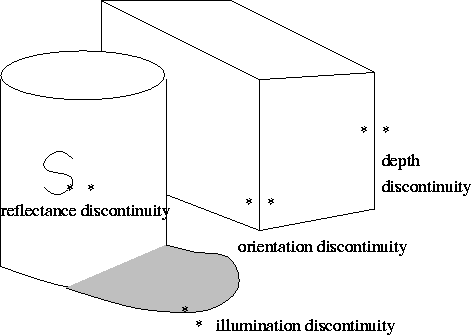
The features that appear in a line drawing may result from a number of different scene events (see figure 1):

• shadow lines correspond to an illumination discontinuity;
• an orientation discontinuity occurs when the surface normal is discontinuous;
• a depth discontinuity occurs at the edge of an object; and
• surface reflectance discontinuities can occur because of surface markings.

 

Figure 1: Image features resulting from different scene events.

Discontinuities in surface normal, illumination, and surface reflectance all lead to viewpoint-independent edges, that is to edges whose three-dimensional spatial locations are independent of the viewpoint. By contrast, continuous surface-normal discontinuities, such as those that occur at the edge of a sphere, correspond to edges whose three-dimensional spatial location depends upon the viewpoint. Such edges are known as limbs or apparent contours.

In this lecture we will assume that the line drawing contains no surface reflectance discontinuities and no illumination discontinuities. Thus, we will only deal with depth and orientation, concentrating on the geometric aspects of the image.

What we would like to do is interpret the surfaces making up the objects in the scene. Clearly, we can't expect to determine functions that describe these surfaces when we only have the boundary information. The best we can hope for is line labeling followed by quantitative shape inference. Line labeling has been solved in general, whereas quantitative shape inference has only been solved for polyhedra.

 

Figure 2: Line labels for concave and convex edges, and for surface normal discontinuities.

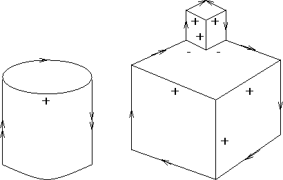
Figure 2 illustrates the six possible labels we can attach to edges. A convex edge is an edge along which the visible angle between the two faces forming the edge is greater than $\pi$. A concave edge is an edge along which the visible angle between the two faces forming the edge is less than $\pi$. An occluding edge is a convex edge along which only one of the two faces adjoining the edge in space is visible in the line drawing. The label $\wedge$ along an occluding edge is so directed that upon looking along the edge in that direction, the body of the object is on your right. Limbs are labeled with $~_{\hat{\hat{~}}}$. Clearly, labeling is not unique, as is evidenced by optical illusions such as the Necker cube.

 

Figure 3: The Necker cube illusion.

Where labels change we have junctions, determined by discontinuous tangents or curvatures. There are six possible labels, giving the label set

$$L = \{+, -, \wedge, \vee, \stackrel{~\wedge}{~_{\wedge}}, \stackrel{~\vee}{~_{\vee}}\}.$$

So with n curves we have 6ⁿ possibilities for assigning labels to the curves. A labeling of a line drawing is a function from L into the set of possibilities. However, it is clear that humans don't consider all possibilities when assigning an interpretation to a line drawing.

Line labels capture the qualitative nature of a line drawing in the sense that bulges in the surface neither change the labeling not the line drawing. We will describe a scheme for labeling line drawings first described by Huffman [3], and independently by Clowes [1], in 1971. Huffman restricted his attention to the case where all faces are planar, that is, a ``polyhedral world'', so now there are only four possible labels $\{+, -, \vee, \wedge \}$. He also assumed that all vertices are trihedral, that is, they are formed by exactly three faces, and that there are no object alignments, which would result in a ``crack'' edge.

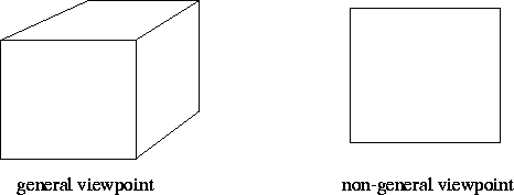
Huffman first noted the need for a general viewpoint assumption, that is, he assumed that the line drawing was viewed from a general viewpoint, so that a small perturbation of the viewpoint would not affect the line drawing. Figure 4 illustrates a general and non-general viewpoint image of a cube.

 

Figure 4: General and non-general views of a cube.

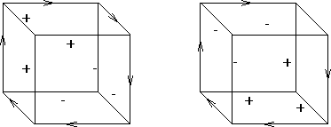
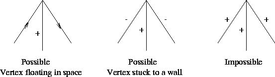
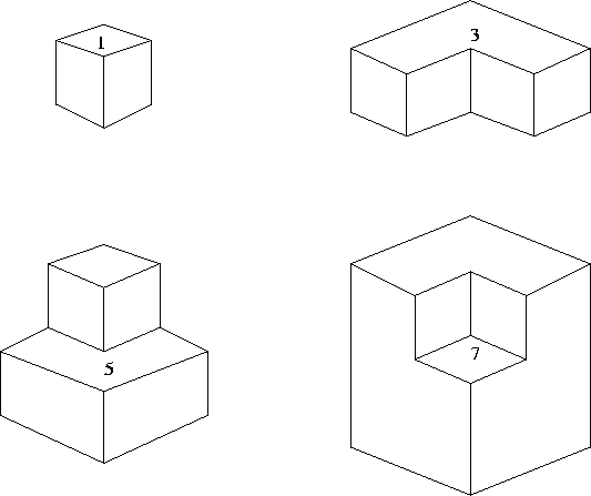
We also note that not all possible line labels lead to legal labelings, that is, to representations of objects that are constructible in the real world. Figure 5 illustrates some legal and illegal labelings.

 

Figure 5: Possible and impossible figures.

Huffman began by constructing all the possible trihedral vertices that could be viewed from all possible viewpoints, thus finding all physically possible junctions. He did this by constructing a cube that was divided in each of the three orthogonal directions. Imagine that any one octant is filled with solid material, and it is then viewed from the other 7 octants. When two octants are filled, we either have a rectangular slab of material which is qualitatively like a single octant cube, or a solid made up from diagonally opposite octants, which is an illegal polyhedron under the Huffman assumptions (the vertices are not all trihedral).

Similar arguments apply when either 4 or 6 octants are filled, so the only interesting cases are filling 1, 3, 5, and 7 octants with solid material, leading to four basic ways in which three planar surfaces can form a vertex of a polyhedron. These are illustrated in figure 6.

 

Figure 6: The four ways of forming trihedral vertices.

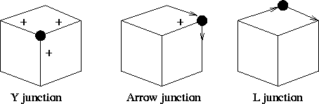
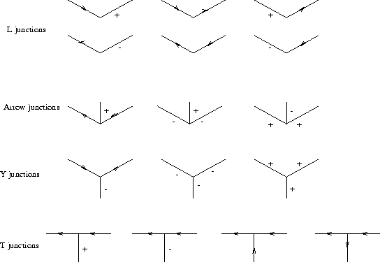
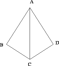
Within each unoccupied subspace, the appearance of the vertex in the line drawing remains the same with respect to the number, the labels, and the configuration of the lines forming that vertex. There are three possible line configurations forming the junction, and they are called Y, L and arrow junctions. The fourth possible junction type is called a T junction, and occurs at depth discontinuities, indicating an occluding boundary. A T junction corresponds to a global scene phenomenon, whereas all the other junction types represent local scene events. An example of the junctions that can be seen from various octants for the case where one octant is filled is given in figure 7. The complete junction catalogue for polyhedral scenes is given in figure 8. Note that simple combinatorics would suggest a much larger junction dictionary; we ought to be able to label in 4³ = 64 distinct ways. But as we saw before, many of these combinations are not physically realizable.

 

Figure 7: The possible views of a cube vertex.

 

Figure 8: The complete junction catalogue.

A line drawing is said to be labelable if a label can be assigned to every segment such that every junction is labeled according to the junction catalogue.

For example, let us label the line drawing shown in figure 9.

 

Figure 9: A line drawing with three possible labelings.

Junctions A and C are arrow junctions, and thus have three possible labelings each. Junctions B and D are L junctions, and thus have six possible labelings each. However, we cannot arbitrarily assign labels within these groups because of global consistency constraints. So we begin by making an arbitrary assignment for A and see how this affects the possible assignments for B, C and D. We will see that there are only three possible interpretations of this line drawing: a tetrahedron on a table, a tetrahedron floating in space, and a tetrahedron stuck on a wall. Thus we ended up with 3 out of 4⁵ = 1024 possibilities.

Huffman checked for labelability by adopting a linguistic approach. Four boolean predicates $\lambda_i^+, \lambda_i^-, \lambda_i^{\rightarrow}, \lambda_i^{\leftarrow}$ are introduced for all segments s_i, where $i = 1 \ldots N$, such that $\lambda_i^+ = 1$if and only if s_i is labeled ``+'', and likewise for $\lambda_i^-$.For $\lambda_i^{\rightarrow}$ and $\lambda_i^{\leftarrow}$, we suppose that an arbitrary direction has been assigned a priori to all segments (this is automatically true if segments are stored as pairs of vertices). Then we pose $\lambda_i^{\rightarrow} = 1 (\lambda_i^{\leftarrow} = 1)$ if and only if s_i is labeled with an arrow that is concordant (discordant) to the intrinsic direction of the segment.

The four predicates must obey the following equation, which assures that exactly one of the predicates is true for all segments:

$$\lambda_i^+ \overline{\lambda}_i^- \overline{\lambda}_i^{\ri... ...\overline{\lambda}_i^{\rightarrow} \lambda_i^{\leftarrow} = 1.$$

Each legal labeling of a junction corresponds to a set of values for the predicates associated with the segments of the junction. This set of values can be described by a boolean equation. For example, the following equation must hold for the predicates of the incident segments s_i, s_j, s_k (arranged in an anti-clockwise direction) of a Y junction (it is assumed that the intrinsic direction of the segments is the outward direction):

$$\lambda_i^+ \lambda_j^+ \lambda_k^+ + \lambda_i^- \lambda_j^... ...lambda_i^{\leftarrow} \lambda_j^- \lambda_k^{\rightarrow} = 1.$$

Now we have an equation for each segment, and an equation for each junction. Putting all these equations together we get a boolean proposition that can easily be put in conjunctive normal form, and is satisfiable if and only if the line drawing is labelable. The labeling problem has therefore been reduced to a satisfiability problem for a boolean expression. Note, thus, that labeling of trihedral scenes, like the satisfiability problem, is $\cal NP$-complete. This linguistic approach to labeling is a very inefficient way of solving the problem.

In 1971 Waltz [8] exhibited a filtering algorithm with very good average running time (roughly linear in the number of segments). The algorithm achieves local consistency in the following way: given a junction, rule out all legal labelings of the junction for which there is no labeling of the neighbour junctions which is compatible with it. Repeat this procedure until no further progress can be made. To label a line drawing, first achieve this local consistency and then achieve global consistency by tree searching with backtracking. Malik [4] applied a similar approach to the labeling of piecewise smooth curved line objects. Parodi [6] has recently studied the complexity of labeling origami scenes, that is scenes constructed by assembling planar panels of negligible thickness, and has shown that this problem is also $\cal NP$-complete.

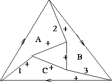
Using schemes such as those above, Escher type objects can be shown to be physically impossible. Hence, all physical objects (in the trihedral world) should be labelable. However, labelability is not a sufficient condition for physical realizability. We can see this with the example illustrated in figure 10. We can visualize this object as a truncated pyramid, where the edges 1, 2 and 3 do not meet at a single point. Such an object is not physically constructible with planes because if it were, then edge 1 would meet face B at some point P. Now P, being a point on edge 1, lies on A and C. Since P meets B, P therefore lies on A and B, implying that P lies on line 2. Likewise, P lies on C and B, implying that P lies on line 3. But we assumed that the edges 1, 2 and 3 did not meet at a single point, so we have a contradiction.

 

Figure 10: A consistent labeling that is not physically realizable.

The realizability problem for a labeled line drawing was solved by Sugihara [7] in 1982. He reduced the problem to an instance of Linear Programming. Roughly speaking, the reduction goes as follows:

• planar faces are represented by the equation of the planes which contain them (a_ix + b_iy + z + c_i = 0), and 3D vertices are represented by a triple v_j = (x_j, y_j, z_j) such that (x_j, y_j) are the 2D coordinates of the corresponding junction;
• whenever, on account of a given labeling, a vertex v_j can be said to lie on face f_i (this is true, for example, if the edge to which v_j belongs is labeled ``+'' or ``-'' and is on the boundary of f_i), the following equation holds true:

  a_ix_j + b_iy_j + z_j + c_i = 0,

  where the unknowns are a_i, b_i, c_i and z_j;
• whenever a vertex v_j can be said to be closer to the centre of projection than the face f_i (this is true if, for example, part of face f_i is occluded by face F_k along an occluding line l and v_j is in the middle of l), the following inequality holds true:

  a_ix_j + b_iy_j + z_j + c_i > 0.

• Now if all the equations, along with all the inequalities, above have solutions, the labeled line drawing correctly represents a polyhedral scene.

Since Linear Programming can be solved in polynomial time, the realizability question can be answered and a possible realization for a labeled line drawing can be exhibited in polynomial time. Thus, realizability can be efficiently checked only when a legal labeling is already available.