Please read the introduction giving general information about the nature of this document.
To use this file, you must be sitting at a colour workstation or X-terminal, running X-windows. Poplog version 14.2 or later must be available.
You should have started Poplog by giving the command
pop11 +popvision %x
in an xterm window. If the popvision saved image is not available, this will produce a warning message. In this case, just start Poplog using
pop11 %x
which will simply mean that the libraries will take a little longer to load.
You should avoid running at the same time any program that displays a lot of different colours, as it may use up too many colour map entries.
It is possible to run all the examples in this file by marking and executing the pieces of indented code, but it is necessary to do this in order from the beginning. You should therefore aim to read this file in one or two sittings.
You might find that at some stage you get the *ROM mishap, which tells you that you need to allow Poplog to use additional memory. If this mishap happens, increase *POPMEMLIM (doing round(1.5 * popmemlim) -> popmemlim would be reasonable) and then carry on by trying again to execute the code segment that was running when the mishap occurred.
Before proceeding further, load the basic libraries that will be needed, by marking the following indented lines and pressing <CTRL-D>. This may take quite a while as external code (i.e. machine code compiled from C rather than a Poplog language) is loaded.
    uses popvision      ;;; search popvision libraries
    uses rci_show       ;;; image display utility
    uses showarray      ;;; array printing utility
    uses arrayfile      ;;; array storage utility
    uses sunrasterfile  ;;; alternative image storage
If you want to know more about these libraries, look at the relevant HELP files (*POPVISION, *RCI_SHOW, *SHOWARRAY and *ARRAYFILE) - but it is not important to do so at this stage.
The first move is to get hold of a representation of an image, and store it in memory so that it is accessible to the Poplog system. For real-time applications, this is done using a special-purpose piece of hardware, called a frame grabber, to digitise a video signal from a TV camera or video tape recorder. However, it is more convenient for now to read a previously digitised image from disc, as follows:
    vars image;             ;;; declare a permanent variable
    arrayfile(popvision_data dir_>< 'stereo1.pic') -> image;
The call to arrayfile sets aside some memory in the form of a Pop-11 array, and then reads data from the named file into the array. The array itself is returned (and assigned to the variable image). The next section examines how arrays are used in Pop-11, but for now, we will use one of the routines loaded above to have a look at the data:
rci_show(image) -> ;

The procedure rci_show creates a new window on the screen and displays the image in it. (It also returns a result, which was discarded as it is unimportant at present.) You can move and iconify the display window as you would any other window. To remove the window entirely, just put the cursor over the image and click any mouse button. You must not (at the time of writing) destroy the display window by selecting an option from its titlebar menu, or you will exit from your Poplog session.
If you have destroyed the image display window, create another one by executing rci_show(image) -> ; again.
Pop-11 arrays are very similar to arrays in other programming languages, and arrays are almost always used to represent images, so although we are using Pop-11, the ideas are very general.
A two-dimensional array can be thought of as being organised as rows and columns. To get any particular value from the array you specify a column and a row. You can picture the layout like this:
            Col  Col  Col  Col  Col  Col
             1    2    3    4    5    6
    Row 1    *    *    *    *    *    *
    Row 2    *    *    *    *    *    *
    Row 3    *    *    *    *    *    *
    Row 4    *    *    *    *    *    *
    Row 5    *    *    *    *    *    *
where each asterisk stands for one data value - in the case of a grey-level image this is typically a number from 0 (dark) to 255 (bright), but other ranges are possible. Sometimes, the symbol X is used to stand for column number, and Y for row number, so that we work in a coordinate system with axes like this:
        +---------------------------> X
        |
        |
        |
        |
        |
        |
      Y V
Note that Y runs the opposite way to conventional coordinates; this is an unfortunate side-effect of the fact that TV systems scan a picture from top to bottom. (It is possible to turn the image over if you want to work in conventional (X, Y) coordinates.)
Arrays in Pop-11 (and most other languages) do not have to start from row 1 and column 1. Try printing the array we read in above, as a Pop-11 object:
    image =>
prints:
    ** <array [80 176 64 191]>
The output tells us that we have an array object, and also what its size and shape are. The list of numbers that follows the word "array" is called the boundslist of the array, and specifies that the column numbers run from 80 to 176, and the row numbers from 64 to 191. (The fact that there are 4 entries in the boundslist says that we have a two-dimensional array.) Graphically, the array has the shape:
                 80     ...    176
                 ------------------
             64  |                |
                 |                |
              .  |                |
              .  |                |
              .  |                |
                 |                |
                 |                |
                 |                |
            191  |                |
                 ------------------
Later we will use boundslist-type structures to specify the bounds of rectangular regions within arrays, so make sure you are familiar with the boundslist ordering: for a 2-D array or region it is
[FIRST-COLUMN LAST-COLUMN FIRST-ROW LAST-ROW].
One element of the array is sometimes called a pixel (for picture element). How many pixels has this array? (Remember that you can use VED as a calculator just by pressing ENTER, typing a colon (:) and then typing in any arithmetic expression and pressing RETURN.) When you have worked out the answer from the array bounds, you can check it by executing
    datalength(image) =>
prints:
    ** 12416
To access a single array element, you treat the array as a procedure, and call it with the column and row numbers as arguments. So to find out the grey-level in the top left corner of our image, execute:
    image(80, 64) =>        ;;; Note: image(COLUMN, ROW)
prints:
    ** 39
This single value is not very informative, but showarray can be used to look at the numerical values of several of the pixels, like this:
    true -> sa_print_axes;    ;;; make showarray show row and col nos
    showarray(image, [80 96 64 70], false, "nums", '');

prints:

   88888888888888888888888888888888888888889999999999999999999999999999
   00001111222233334444555566667777888899990000111122223333444455556666

64>  39  39  42  50  55  55  52  75 108 117 105 101 102 105 106 104 102
65>  45  45  45  48  60  57  55  74 107 112 107 104 105 106 102 100  99
66>  42  37  30  33  43  47  51  74 113 117 103  99  96  94  98 103 108
67>  48  44  39  40  47  51  54  83 123 128 108 101  99  95  99 102 106
68>  39  36  33  34  43  50  48  75 107 112  98 100 105 106 104 103  99
69>  41  41  37  45  42  45  50  77 107 111 101  98 104 104 106 109 106
70>  32  29  24  29  29  38  52  81 118 125 108 103  99  94  96 102 101
This prints out the values for columns 80 to 96 and rows 64 to 70. The column and row numbers appear as well (the column numbers have to be read downwards). You can see how the grey-level values change as you go from left to right across the first two vertical stripes at the top left of the image. Look at the structure of the edge between the stripes (around column 87) - it looks sharp on the screen, but how rapidly do the values change from one pixel to the next?
We can display the region of the image whose grey-levels we have printed out at a larger scale, in order to see the individual pixel structure. The following code will do this - do not worry for now about the details of the arraysample procedure, but note the boundslist-type argument which is used to pick out a small region of the the array.
    10 -> rci_show_scale;           ;;; increase the scale
    rci_show(arraysample(image, [80 96 64 70], false, false, "nearest"))
            -> ;
    1 -> rci_show_scale;            ;;; put the scale back as it was

You may need to move the newly-created window with the mouse so that it does not obscure the window containing the original image.
The rci_show procedure adjusts its display so that the highest grey-level in the window appears white and the lowest appears black. For that reason, the brightnesses in the new window will not correspond exactly to the brightnesses in the top left corner of the old display window, though the relative brightnesses within the windows will be the same. (It is possible to change this behaviour, but it is not important to look into this at present.)
You should now be clear about how array indices (the numbers used to refer to an array element, such as 80,64 above) correspond to positions in the image represented by the array, and you should also understand the meaning of the boundslist of the array. For more technical details about Pop-11 arrays, see HELP *ARRAYS and REF *ARRAYS.
You have also been introduced to two display tools - rci_show and showarray - and one image manipulation utility - arraysample. When you want to use these procedures for your own purposes you may need to refer to their associated help files.
To change the value stored at a particular location in an array, you again treat the array as a procedure, and use its updater. So the following code will create a small white square in our image, destroying some of the original data:
    255 ->> image(90,66) ->> image(90,67) ->> image(90,68)
        ->> image(91,66)                  ->> image(91,68)
        ->> image(92,66) ->> image(92,67) ->> image(92,68);
Now display the array again using rci_show, and notice the new white square near the top left corner. Use the example above to view it at 10x enlargement as well as at normal scale.


(Note, incidentally, that if you just want to superimpose graphics on top of an image, you should not do it like this - use the *RC_GRAPHIC facilities instead.)
Suppose we had wished to change the array without destroying any of the original data. Sometimes people try to do something like this:
    vars newimage;
    image -> newimage;              ;;; copy the image (???)
    vars column;
    for column from 110 to 140 do
        255 -> newimage(column, 140);     ;;; change the new array
        255 -> newimage(column, 142);     ;;; change the new array
        255 -> newimage(column, 144);     ;;; change the new array
    endfor;
The for loop is just some arbitrary code to change the array in a way that will be visible. Note that it updates newimage rather than image.
This strategy does not work. If you execute the code above and then display the "original" image with
rci_show(image) -> ;

you will see white lines across the picture, caused by assigning the value 255 to some of the pixels.
The reason for this is that the assignment image -> newimage does not create a new array; it simply causes the variable newimage to refer to the original array. Both image and newimage then refer to this one data structure. Since there is only one array, changes to it are seen whichever way you access it. If you do not understand this, you should review your work on variables and data structures, perhaps by reference to material from your earlier Pop-11 courses.
The correct way to do what we want is in fact very simple. Instead of writing
image -> newimage;
we should have written
copy(image) -> newimage;
which will create a new array and copy the data into it (see HELP *COPY). The variables image and newimage will then refer to completely different objects, and changing one of these will not affect the other. You should verify this by modifying the code above and displaying the two different arrays. (You should change the position of the lines of white pixels so that you can be clear about what effect you have had on the arrays).
Many bugs are caused by programmers sometimes forgetting that assignments (including assignments to arguments during procedure calls) do not copy data structures.
So far you have seen three ways of creating new arrays: using arrayfile, copy and arraysample. It is also possible to create a new array, and initialise its contents, with a call to one of the explicit constructor procedures newarray and newanyarray. These are described in the relevant REF and HELP files, and in Pop-11 textbooks - they take a boundslist as an argument and return an array. For vision applications it is sometimes useful to create special kinds of arrays with newsarray and newsfloatarray.
This final section gives an example of a simple image processing program.
Significant features of an image often correspond to large changes in the grey-level between neighbouring pixels. A boundary in the image, provided it is not horizontal, will result in grey-level changes between pixels in the same row and in neighbouring columns. Let us look at the sizes of such changes for all the pixels in our image, as a possible first step to extracting more useful structure from the image.
To do this, we will take each pixel in turn, using for loops to go through the whole of the array. For each pixel, we subtract the value of the pixel in the next column to the left. If, at the pixel in question, the image gets brighter going left to right, the result will be positive; if the image gets darker the result will be negative; if the brightness is fairly uniform the result will be close to zero.
To try this, first set up an output array in which to store the results. Since there is nothing to subtract from the left-most pixel in each row, the output array should start from column 81 instead of column 80.
newarray([81 176 64 191]) -> newimage;
Now we can set up two loop variables and then iterate over the original array, doing the subtractions:
    vars row, column;           ;;; loop variables
    for row from 64 to 191 do
        for column from 81 to 176 do
            image(column, row) - image(column-1, row)
                -> newimage(column, row)
        endfor
    endfor;
You should be certain that you understand this code fragment. It is typical of low-level vision programs.
Having executed this code, display the results. They will be clearer if we use a larger scale:
    2 -> rci_show_scale;            ;;; double the scale
    rci_show(image) -> ;            ;;; redisplay the original image
    rci_show(newimage) -> ;         ;;; display the processed image

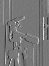
You may need to move the display of the processed image with the mouse to see the original image.
Note how the vertical boundaries stand out as dark or bright regions in the new image, corresponding to the positive and negative values in the difference array that has been created. Zero appears as a mid-grey in this display (though you can change this behaviour - see *RCI_SHOW should you want to do so.)
We can also check a few of the values using showarray:
    showarray(newimage, [81 90 64 70], false, "nums", '');

prints:

   88888888888888888888888888888888888888888888899999
   11111222223333344444555556666677777888889999900000

64>    0    3    8    5    0   -3   23   33    9  -12
65>    0    0    3   12   -3   -2   19   33    5   -5
66>   -5   -7    3   10    4    4   23   39    4  138
67>   -4   -5    1    7    4    3   29   40    5  127
68>   -3   -3    1    9    7   -2   27   32    5  143
69>    0   -4    8   -3    3    5   27   30    4  -10
70>   -3   -5    5    0    9   14   29   37    7  -17
where at the top left we have 39 - 39 = 0, 42 - 39 = 3, 50 - 42 = 8, etc.
You should now modify the code above to display the vertical rather than horizontal differences, and hence highlight horizontal rather than vertical boundaries.
The code above is, of course, an illustrative fragment, and is not suitable for incorporating into a serious program because the size of the array we happen to be using has been built into it. For any real application, the differencing code would be made into a general procedure, which might look like this:
    define hordiffs(image) -> newimage;
        ;;; Returns a new array. Each pixel of the result holds a
        ;;; horizontal difference between two neighbouring pixels
        ;;; of the input array.
        lvars image, newimage;
        lvars row, column, colstart,
            (col0, col1, row0, row1) = explode(boundslist(image));
        ;;; Cannot calculate output for LH column
        col0 + 1 -> colstart;
        newarray([% colstart, col1, row0, row1 %]) -> newimage;
        for row from row0 to row1 do
            for column from colstart to col1 do
                image(column, row) - image(column-1, row)
                    -> newimage(column, row)
            endfor
        endfor
    enddefine;
which if you load it can be tested with
rci_show(hordiffs(image)) -> ;

Note how boundslist is used to set up the loop limits, and how the issue of the left-hand column is handled, without any extraneous tests inside the loops. (Some programmers put tests in the loops to avoid accessing pixels outside the array bounds, but this is extremely inefficient.) Note also that all the local variables (including the arguments) are declared as lvars for efficiency and modularity.
Many low-level operations in computer vision are related to this example. It is, in fact, a special case of a process known as convolution, which we will examine more fully later.
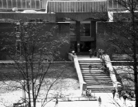
You may get tired of looking at the image of the tripod head. A few other images are available, and you could experiment with these. They are read using *sunrasterfile instead of arrayfile; for example:
sunrasterfile(popvision_data dir_>< 'mtg_ho.ras') -> image;
To get a list of the images currently available in the system, find the name of the data directory with
popvision_data =>
and then list it with
<ENTER> ls dir
where dir is the directory printed out as the value of popvision_data.
Once read into arrays, these other images can be used as alternatives to stereo1 in all the teach files except for the one on stereoscopic vision; however, as they are larger they will take longer to process, so at busy times it is better to stick with stereo1.
You should now:
Here are links to:
Copyright University of Sussex 1994. All rights reserved.