Common Names: Contrast stretching, Normalization
Contrast stretching (often called normalization) is a simple image enhancement technique that attempts to improve the contrast in an image by `stretching' the range of intensity values it contains to span a desired range of values, e.g. the the full range of pixel values that the image type concerned allows. It differs from the more sophisticated histogram equalization in that it can only apply a linear scaling function to the image pixel values. As a result the `enhancement' is less harsh. (Most implementations accept a graylevel image as input and produce another graylevel image as output.)
Before the stretching can be performed it is necessary to specify the upper and lower pixel value limits over which the image is to be normalized. Often these limits will just be the minimum and maximum pixel values that the image type concerned allows. For example for 8-bit graylevel images the lower and upper limits might be 0 and 255. Call the lower and the upper limits a and b respectively.
The simplest sort of normalization then scans the image to find the lowest and highest pixel values currently present in the image. Call these c and d. Then each pixel P is scaled using the following function:
Values below 0 are set to 0 and values about 255 are set to 255.
The problem with this is that a single outlying pixel with either a very high or very low value can severely affect the value of c or d and this could lead to very unrepresentative scaling. Therefore a more robust approach is to first take a histogram of the image, and then select c and d at, say, the 5th and 95th percentile in the histogram (that is, 5% of the pixel in the histogram will have values lower than c, and 5% of the pixels will have values higher than d). This prevents outliers affecting the scaling so much.
Another common technique for dealing with outliers is to use the intensity histogram to find the most popular intensity level in an image (i.e. the histogram peak) and then define a cutoff fraction which is the minimum fraction of this peak magnitude below which data will be ignored. The intensity histogram is then scanned upward from 0 until the first intensity value with contents above the cutoff fraction. This defines c. Similarly, the intensity histogram is then scanned downward from 255 until the first intensity value with contents above the cutoff fraction. This defines d.
Some implementations also work with color images. In this case all the channels will be stretched using the same offset and scaling in order to preserve the correct color ratios.
Normalization is commonly used to improve the contrast in an image without distorting relative graylevel intensities too significantly.
We begin by considering an image
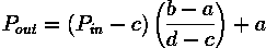
which can easily be enhanced by the most simple of contrast stretching implementations because the intensity histogram forms a tight, narrow cluster between the graylevel intensity values of 79 - 136, as shown in
After contrast stretching, using a simple linear interpolation between c = 79 and d = 136, we obtain
Compare the histogram of the original image with that of the contrast-stretched version
While this result is a significant improvement over the original, the enhanced image itself still appears somewhat flat. Histogram equalizing the image increases contrast dramatically, but yields an artificial-looking result
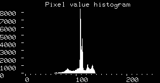
In this case, we can achieve better results by contrast stretching the image over a more narrow range of graylevel values from the original image. For example, by setting the cutoff fraction parameter to 0.03, we obtain the contrast-stretched image
and its corresponding histogram
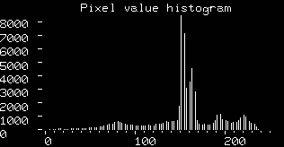
Note that this operation has effectively spread out the information contained in the original histogram peak (thus improving contrast in the interesting face regions) by pushing those intensity levels to the left of the peak down the histogram x-axis towards 0. Setting the cutoff fraction to a higher value, e.g. 0.125, yields the contrast stretched image
As shown in the histogram
most of the information to the left of the peak in the original image is mapped to 0 so that the peak can spread out even further and begin pushing values to its right up to 255.
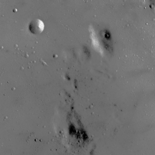
As an example of an image which is more difficult to enhance, consider
which shows a low contrast image of a lunar surface.
The image
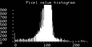
shows the intensity histogram of this image. Note that only part of the y-axis has been shown for clarity. The minimum and maximum values in this 8-bit image are 0 and 255 respectively, and so straightforward normalization to the range 0 - 255 produces absolutely no effect. However, we can enhance the picture by ignoring all pixel values outside the 1% and 99% percentiles, and only applying contrast stretching to those pixels in between. The outliers are simply forced to either 0 or 255 depending upon which side of the range they lie on.
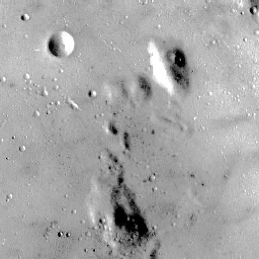
shows the result of this enhancement. Notice that the contrast has been significantly improved. Compare this with the corresponding enhancement achieved using histogram equalization.
Normalization can also be used when converting from one image type to another, for instance from floating point pixel values to 8-bit integer pixel values. As an example the pixel values in the floating point image might run from 0 to 5000. Normalizing this range to 0-255 allows easy conversion to 8-bit integers. Obviously some information might be lost in the compression process, but the relative intensities of the pixels will be preserved.
You can interactively experiment with this operator by clicking here.
(You must begin by selecting suitable values for c and d.) Next, edge-detect (i.e. using the Sobel, Roberts Cross or Canny edge detector) both the original and the contrast stretched version. Does contrast stretching increase the number of edges which can be detected?
E. Davies Machine Vision: Theory, Algorithms and Practicalities, Academic Press, 1990, pp 26 - 27, 79 - 99.
A. Jain Fundamentals of Digital Image Processing, Prentice-Hall, 1989, Chap. 7, p 235.
D. Vernon Machine Vision, Prentice-Hall, 1991, p 45.
Specific information about this operator may be found here.
More general advice about the local HIPR installation is available in the Local Information introductory section.
©2003 R. Fisher, S. Perkins,
A. Walker and E. Wolfart.
![]()