This page explains the theory behind solving networks of queues. Queueing networks fall into two main categories - open and closed. Open networks receive customers from an external source and send them to an external destination. Closed networks have a fixed population that moves between the queues but never leaves the system. We will now refer to single queues, as described in the previous section, as service centres. Service centres in a network exhibit the same behaviour as single queues. First we will discuss open networks. An example of an open network is shown in Figure 1.
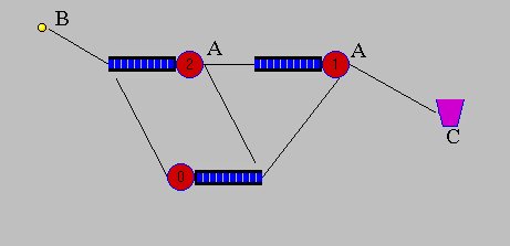
Figure 1: An Open Queueing Network
The yellow circle, B, represents an external source of customers. There are three inter-connected service centres and an external destination,C. Each service centre has a mean service time. When a customer leaves a service centre there may be more than one possible destination (eg at places marked A on the diagram). It is therefore necessary to define routing probabilities. This is done by attaching a weighting to each possible destination. For example upon leaving queue 2, there are two possible destinations - queue 1 and queue 0. If both of these destinations had weight 1 then there would be an equal probability of a departing customer going to either queue. However, if queue 1 had weight 1 and queue 0 had weight 2, then, on average, one in three customers would go to queue1 and two in three customers would go to queue 0. To solve the network and determine performance measures for each queue one solves the Traffic Equations for the network. This allows us to find the effective arrival rate at each queue and then using the methods of the previous page we can determine performance measures for each queue. It is possible to design your own open queueing networks using the applet below. See the Instructions for further details.
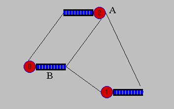
Figure 2: A Closed Queueing Network
Closed queueing networks do not have a source or sink. An example of a closed network is shown in Figure 2. The service centres perform as in the open network case and routing probabilities are defined in the same way (eg. at A on the diagram). When one builds a closed network it is necessary to define the number of customers which are initially in each of the service centres. These customers can then travel around the network but cannot leave it. To solve a closed network, we again have to solve the Traffic Equations. However, we do not have an external arrival rate to allow us to solve the equations completely so we have to define the throughput of one of the queues as 1 and then express the throughput of the other queues relative to this reference queue. Having solved the traffic equations it is possible to determine measures for the network by using Mean Value Analysis. You can design your own closed queueing networks using the applet below and it will use MVA to determine measures such as the mean number of customers in each service centre and also the mean waiting time of a customer at each service centre.
Design, solve and simulate your own queueing networks using the applet below. Press 'Instructions' for more help.
The traffic equations are used to determine the throughput/effective arrival rate of each of the queues in a network. Here we will look at the traffic equations of a simple open network. The ideas are easily extended to more complex open networks and to closed networks (with the throughput of one queue normalised to one and all other throughputs expressed relative to that reference queue). The network we will consider is shown in Figure 3. The number beside each service centre is the service time for that service centre. The numbers beside the connections are the routing probabilities (normalised so as they sum to one for the sake of this example - note that the applet above must have integer weightings).
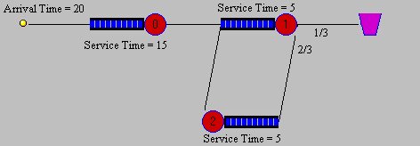
Figure 3. Open Network Diagram
We consider each queue in turn and write an equation for its throughput.
Queue 0: The only input to queue 0 is the source so its throughput is just the arrival rate from the source ie 1/20. So the first traffic equation is: X0 = 1/20.
Queue 1: This queue has no direct input from the source and thus we can only express its throughput in terms of the throughput of those queues which lead into it ie. X1 = X0 + X2.
Queue 3: This has input from only one queue, namely queue 1. It only gets 2/3 of the customers that leave queue 1 so we can write this as X2 = 2/3.X1.
So we have three equations in three unknowns which can be solved using standard linear algebra techniques. For this example we get: X0 = 0.05, X1 = 0.15, X2 = 0.1.
This method would be equally effective with more queues and more complex connections. Try designing your own networks and pressing the 'Traffic Equations' button.
This method uses a number of fundamental queueing relationships to determine the mean values of throughput, delay and queue size for closed queueing networks which have 'product form'.
Suppose we have a queueing network with M queues and N customers and that the ith queue has service rate ui. Let ti be the average delay that a customer experiences at the ith queue. Then ti has two parts - the time spent waiting in the queue and the time taken to be served:
ti = 1/ui + 1/ui.(mean number of customers present upon arrival).
What is the 'mean number of customers present upon arrival'? It is the mean number of customers at that queue when there is one less customer in the network ie N-1 customers. Let ni(N) be the mean number of customers at the ith queue when there are N customers in the network. Then we can write:
ti = 1/ui + (ni(N-1))/ui
Little's Law states that X=N/W where X = throughput of the network and
W = mean time spent in the network by a job = t1(N) + t2(N) + ... + tm(N).
Let X(N) be the throughput of the network when there are N customers present. Then substituting into Little's law for the entire network gives us:
N = X(N)(t1(N) + t2(N) + ... +tm(N)).
And applying to an individual queue gives:
X(N).ti(N) = ni(N)
Rearranging these equations and adding in routing probabilities oi gives us the following system of equations which can be repeatedly solved to calculate measures for the required number of customers.
ni(0) = 0 i = 1,2,...,M
ti(N) = 1/ui + ni(N-1)/ui i = 1,2,...,M
X(N) = N/(o1t1(N) + o2t2(N) + ... + oMtM(N)) Note: this is the throughput of the reference queue
ni(N) = X(N)oiti(N)
This method is implemented in the applet and the results displayed in 'Calculated Measures' window when 'Submit(Closed)' is pressed.