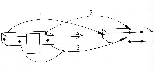
This process starts with the region graph described in Chapter 3. Initially, the surface hypotheses are identical to the image regions. From these, larger surface hypotheses are created based on surface extensions consistent with presumed occlusions. While it is obviously impossible to always correctly reconstruct obscured structure, often a single surface hypothesis can be created that joins consistent visible surface parts. Figure 4.1 shows a simple case of surface reconstruction.
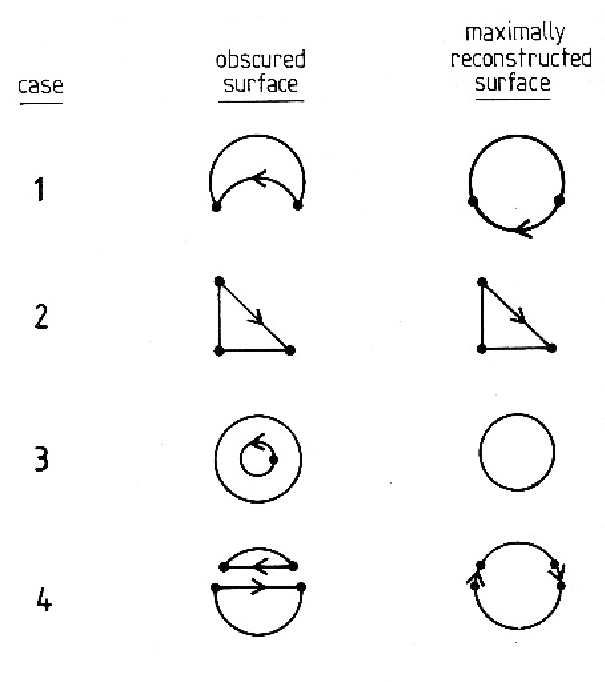
In Figure 4.2, four cases of a singly obscured surface are shown, along with the most reasonable reconstructions possible, where the boundary arrows indicate an occlusion boundary with the object surface on the right of the arrow and the obscuring surface on the left. In the first case, the original surface boundaries meet when they are extended, and this is presumed to reconstruct a portion of the surface. If the boundaries change their curvature or direction, then reconstruction may not be possible, or it may be erroneous. (Even if erroneous, the reconstructed surface may more closely approximate the true surface than the original input.) The second case illustrates when reconstruction does not occur, because the unobscured boundaries do not intersect when extended. The third case shows an interior obscuring object removed. The fourth case shows where the surface has been split by an obscuring object and reconstructed. The label of the boundary extension always remains back-side-obscuring, because it might participate in further reconstructions.
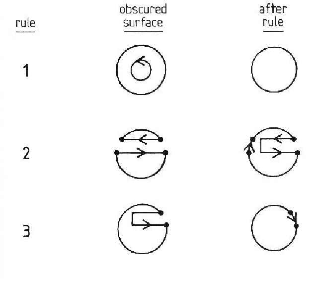
What is interesting is that only three rules are needed for the reconstruction (see Figure 4.3). They are:
Rule 2 connects two separated surfaces if either extension of the boundaries intersect. The remaining portion of the obscuring boundary is disconnected to indicate no information about the obscured portion of the surface (until Rule 3). Rule 3 removes notches in surfaces by trying to find intersecting extensions of the two sides of the notch. Repeated application of these rules may be needed to maximally reconstruct the surface.
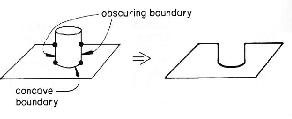
Reconstruction is attempted whenever surface occlusion is detected, which is indicated by the presence of back-side-obscuring labeled boundaries. Concave orientation discontinuity labelled boundaries may also mean occlusion. In Figure 4.4, the base of the obscuring cylinder rests on the plane and so has a concave shape boundary, which should be treated as part of the delineation of the obscured region of the plane. (If the two objects were separated slightly, an obscuring boundary would replace the concave boundary.) As the concave boundary does not indicate which object is in front, it is assumed that either possibility could occur.
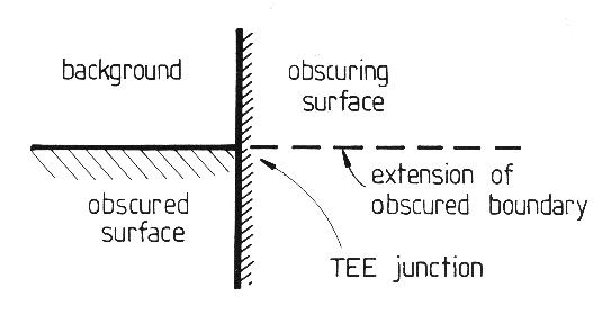
Figure 4.5 shows a typical case where one surface sitting on another will create a TEE junction, or connect to an obscuring boundary (as in Figure 4.4).
After finding the segments indicating occlusion, the points where reconstruction can start need to be found. These are the ends of boundary segments that satisfy:
For reconstruction, boundary segments must intersect when extended. As intersecting three dimensional surface curves still intersect when projected onto the image plane, extension and intersection is done only in two dimensions, thus avoiding the problems of three dimensional curve intersection. Extending the boundaries is done by estimating the curvature shortly before the terminating TEE and projecting the curve through the TEE. On the basis of the boundary segmentation assumptions (Chapter 3), segments can be assumed to have nearly constant curvature, so the extension process is justified. Segments that intersect in two dimensions can then be further tested to ensure three dimensional intersection, though this was not needed when using the additional constraints given below. Further, because of numerical inaccuracies in the range data, three dimensional intersection is hard to validate.
To prevent spurious reconstructions that arise in complex scenes with many obscuring objects, other constraints must be satisfied:
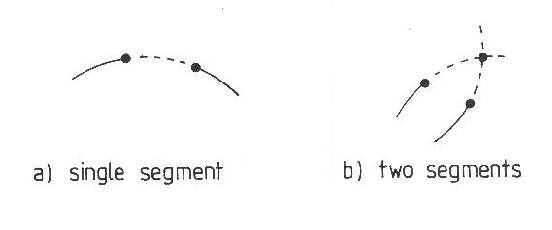
There are two outputs from the reconstruction process - the boundaries and the surface itself. Because of the surface segmentation assumption, the reconstructed surface shape is an extension of the visible surface's shape. The boundary is different because, in the absence of any knowledge of the object, it is impossible to know exactly where the boundary lies. It is assumed that the obscured portion of the boundary is an extension of the unobscured portions, and continues with the same shape until intersection. The two cases are shown in Figure 4.7. In case (a), a single segment extension connects the boundary endpoints with the same curvature as the unobscured portions. In case (b), the unobscured portions are extended until intersection.
The process may incorrectly merge surface patches because of coincidental
alignments, though this is unlikely to occur because of the constraints of
boundary intersection and labeling and surface shape compatibility.
Hence, the conservative approach to producing surface hypotheses
would be to allow all possible surface reconstructions,
including the original surface without any extensions.
This proliferates surface hypotheses causing
combinatorial problems in the later stages.
So, the final surface hypotheses are made from
the maximally reconstructed surfaces only.
If the reconstructed surface is larger than the true surface,
invocation may be degraded, but hypothesis
construction
would continue because
the surface extension is not used.
Verification avoids this problem by using the original image regions
as its input.
The Surface Hypothesis Graph
The region graph (Chapter 3) forms the initial input into the explicit surface hypothesis process. The surface hypothesizing process makes the following additions to the region graph to form the surface hypothesis graph: