Boundary Curvature

The calculation of three dimensional boundary curvature is trivial - the difficulty lies in grouping the boundary segments into sections that might belong to the same feature. Fortunately, the input boundary is labeled with both the type of the segmentation boundary (between surfaces) and the type of discontinuities along the boundary (Chapter 3). This allows sections to be grouped for description with the goal of finding segments that directly correspond to model boundary segments.

Boundaries are not arbitrary space curves, but are associated with surfaces. Hence, the surface determines which boundary sections will be described. Boundaries labeled as:

• convex shape discontinuity boundaries are true object features, and are thus described.
• concave boundaries may be true surface boundaries or may occur where one object rests on another; in either case they are described.
• $<$back-side-obscuring$>$ are definitely not true object boundaries (relative to the current surface) and are not described.
• $<$front-side-obscuring$>$ boundaries may be either orientation discontinuities or extremal boundaries; in either case they are described.

The ring of boundary segments surrounding a surface is partitioned into describable sections by the following criteria:

1. If a segment has the label $<$back-side-obscuring$>$, then it is deleted.
2. If the point where two segments join is labeled as a boundary segmentation point, then split the ring at this point.
3. If two adjacent boundary segments have different labels, then split the ring at their junction point.

Each set of connected boundary segments that remain after the splitting process is described.

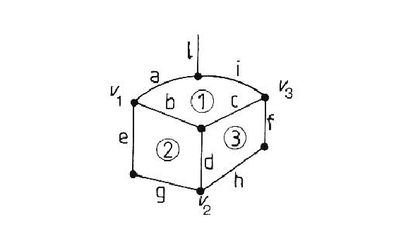
For example, assume that the object in Figure 6.1 is sitting on a surface, that it is a box with an opening at surface 1, that boundary segment l belongs to the background and that the labelings are:

$$\vbox{\vskip 0.5in \hskip 1in \begin{tabular}{ccl} SEGMENT& S... ...-obscuring$>$ \\ l & ? & any \\ \end{tabular}\vskip 0.25in }$$

$$\vbox{\vskip 0.25in \hskip 1in \begin{tabular}{cl} VERTEX& SE... ...tinuity) \\ rest & irrelevant \\ \end{tabular}\vskip 0.25in }$$

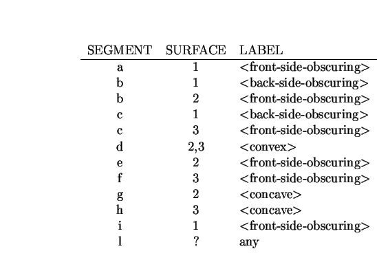
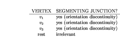
Then, the only describable boundary section for surface 1 is {a,i}. As b and c are $<$back-side-obscuring$>$, they are not used. Segments a and i are not separated by any criterion, so are treated as a single section. For surface 2, each segment is isolated. Between b and d the label changes, as between e and g. Between b and e there is a boundary segmentation point (placed because of an orientation discontinuity in the boundary), as between d and g. Surface 3 is similar to surface 2.

Figure 6.1: Boundary Segment Grouping Example

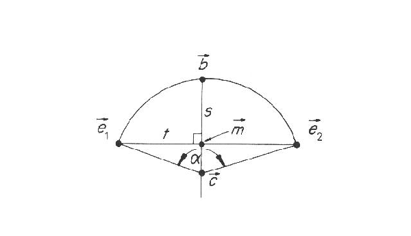
One goal of the boundary segmentation described in Chapter 3 was to produce boundary sections with approximately uniform curvature character. Hence, assuming a boundary section is approximately circular, its curvature can be estimated as follows (referring to Figure 6.2):

Let:
	$\vec{e_1}$ and $\vec{e_2}$ be the endpoints of the section
	$\vec{b}$ be the bisecting point of the section
	$\vec{m}$ be the midpoint of the bounding chord = $( \vec{e_1} + \vec{e_2}) / 2$
If:
	$\vec{m} = \vec{b}$, then the segment is straight,
Otherwise:
	$s = \mid \vec{m} - \vec{b} \mid$
	$t = \mid \vec{m} - \vec{e_1} \mid$
And:
	$curvature = 2s / ( s^2 + t^2 )$

Figure 6.2: Radius Estimation Geometry

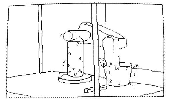
A heuristic declares nearly straight segments as straight. The curvature estimates for some of the complete boundaries in the test image (using segment labels shown in Figure 6.3) are given in Table 6.1.

Table 6.1: Boundary Curvature Estimates

REGION	SEGMENTS	ESTIMATED CURVATURE	TRUE CURVATURE
26	1	0.131	0.125
26	2	0.120	0.125
8	3,4,5	0.011	0.0
8	6	0.038	0.111
8	7,8,9,10	0.010	0.0
9	11,12	0.0	0.0
9	13	0.083	0.090
9	14,15,16	0.012	0.0
9	17,18,19,20	0.054	0.069

Figure 6.3: Test Image Boundary Numbers

The estimation of curvature is accurate to about 10%. Some straight lines have been classified as slightly curved (e.g. segments 3-4-5) but they received large radius estimates (e.g. 90 cm). Some curvature errors arise from point position errors introduced during surface reconstruction. This factor particularly affects boundaries lying on curved surfaces.