Given surface orientation and some elementary geometry, it is possible to estimate the angle at which two surfaces meet (defined as the angle that the solid portion of the junction subsumes). This description is useful for two reasons: (1) extra information is always useful for recognition and (2) the measurement is dependent on the surface's relationship with its neighbors, whereas many other descriptions relate only to the structure in isolation. Hence, context can enhance the likelihood of identification.
This description is only applied to surfaces that are adjacent across a shape boundary and so emphasizes group identification. (Surfaces across an obscuring boundary may not be related.)
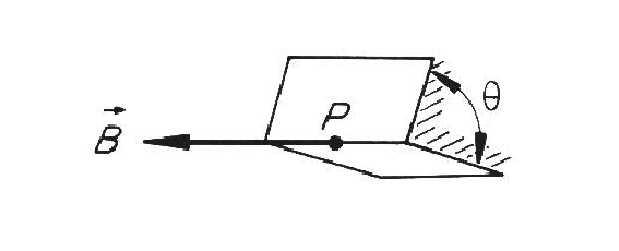
The factors involved in the description's calculation are the orientation of the surfaces, the shared boundary between the surfaces and the direction to the viewer. As the boundary is visible, the viewer must be in the unoccupied space sector between the two surfaces.
Because surfaces can be curved, the angle between them may not be constant along the boundary; however, it is assumed that this angle will not vary significantly without the introduction of other shape segmentations. Consequently, the calculation obtained at a nominal point is taken to be representative.
Figure 6.13 shows two surfaces meeting at a boundary.
Somewhere along this boundary a nominal point ![]() is chosen and also
shown is the vector of the boundary direction at that point (
is chosen and also
shown is the vector of the boundary direction at that point (![]() ).
Through this point a cross-section plane is placed, such that the
normals (
).
Through this point a cross-section plane is placed, such that the
normals (![]() ) for the two surfaces lie in the plane.
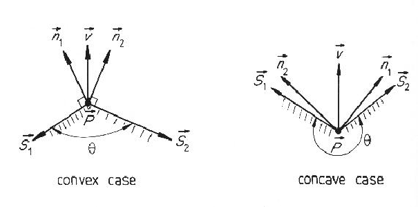
Figure 6.14 shows the two cases for this cross-section.
) for the two surfaces lie in the plane.
Figure 6.14 shows the two cases for this cross-section.
The essential information that determines the surface angle is the
angle at which the two normals meet.
However, it must also be determined whether the surface junction is
convex or concave,
which is the difficult portion of the computation.
The details of the solution are seen in Figure 6.14.
Let vectors ![]() and
and ![]() be tangential to the respective
surfaces in the cross-section plane.
By definition, the vector
be tangential to the respective
surfaces in the cross-section plane.
By definition, the vector ![]() is normal to the plane
in which the
is normal to the plane
in which the ![]() and
and ![]() vectors lie.
Hence, each individual
vectors lie.
Hence, each individual ![]() vector is normal to both the corresponding
vector is normal to both the corresponding
![]() vector and the
vector and the ![]() vector, and can be calculated by a cross product.
vector, and can be calculated by a cross product.
These ![]() vectors may face the wrong direction (e.g. away from
the surface).
To obtain the correct direction, a track is made from the point
vectors may face the wrong direction (e.g. away from
the surface).
To obtain the correct direction, a track is made from the point ![]() in the direction of both
in the direction of both ![]() and
and ![]() .
One of these should immediately enter the surface region, and this is
assumed to be the correct
.
One of these should immediately enter the surface region, and this is
assumed to be the correct ![]() vector.
vector.
Because the boundary must be visible, the angle between the vector
![]() from the nominal point to the viewer
and a surface vector
from the nominal point to the viewer
and a surface vector ![]() must be less than
must be less than ![]() .
Hence, the angle between these vectors is guaranteed to represent open space.
Then, the angle between the two surfaces is
.
Hence, the angle between these vectors is guaranteed to represent open space.
Then, the angle between the two surfaces is ![]() minus these two open spaces.
This computation is summarized below:
minus these two open spaces.
This computation is summarized below:
| Let: | |
| Then, the boundary vector |
|
|
|
|
| and the surface vectors |
|
|
|
|
which are then adjusted for direction, as described above.
Given this, the surface angle is:
The true and estimated surface angles for the modeled objects
are summarized in Table 6.10.
Further, only rigid angles between surfaces in the same primitive
surface clusters are reported (these being the only evidence
used).
The estimation procedure is accurate for orientation discontinuities. The major source of errors for this process is the measurement of the surface orientation vectors by hand, and interpolating their value to the nominal point. This contributed substantially to the error at the curvature discontinuity, where interpolation flattened out the surface.