The Geometric Model

The model is what the system knows about an object. Paraphrasing Binford [29]: a capable vision system should know about object shape, and how shape affects appearance, rather than what types of images an object is likely to produce. Geometric models explicitly represent the shape and structure of an object, and from these, one can (1) deduce what features will be seen from any particular viewpoint and where they are expected to be and (2) determine under what circumstances a particular image relationship is consistent with the model. Both of these conditions promote efficient feature selection, matching and verification. Hence, this approach is intrinsically more powerful than the property method, but possibly at the expense of complexity and substantial computational machinery. However, a practical vision system may also incorporate redundant viewer-centered descriptions, to improve efficiency.

The geometric body model used here introduces a uniform level of description suitable for a large class of objects (especially man-made). It specifies the key primitive elements of an object representation, and how they are positioned relative to the whole object.

Some Requirements on the Model

The models should emphasize the relevant aspects of objects. As this research is concerned with model shape and structure, rather than reflectance, these are: surface shape, intersurface relationships (e.g. adjacency and relative orientation), surface-object relationships and subcomponent-object relationships. To recognize the objects in the test scene, the geometric models will have to:

• make surface information explicit - to easily match image surface data,
• have three dimensional, transformable object-centered representations - because objects can take arbitrary, unexpected spatial locations and orientations,
• have geometric subcomponent relationships - because of the structuring of the surface clusters and the physical constraints on their placement,
• represent solid and laminar objects - to handle the variety in the scene and
• have attachments with degrees-of-freedom - for recognizing articulated objects (e.g. the robot).

These are general requirements; more specific requirements for geometric information are discussed below.

As model invocation (Chapter 8) is based on both image property evidence and component associations, it additionally needs:

• size, shape and curvature parameters of individual surfaces and boundary segments,
• non-structural object relations, such as subtype or subclass,
• adjacency of surfaces and their relative orientation and
• typical configurations of visible components.

Hypothesis construction and verification (Chapters 9 and 10) instantiate and validate invoked models by pairing image data or previously recognized objects with model components. To build the hypotheses, the matcher will have to search the image and its results database for evidence. Verification ascertains the soundness of the instantiated models by ensuring that the substructures have the correct geometric relationship with each other and the model as a whole, and that the assembled object forms a valid and compact solid. Together, the two processes require:

• the type of substructures needed and
• the geometric relationships between the substructures and the object.

Model Primitives

Model surfaces and boundaries are usually segmented according to the same criteria discussed in Chapter 3 for image data (essentially shape discontinuities). Hence, the same primitives are also used for the models to reduce the conceptual distance to the data primitives, and thus simplify matching. The primitive element of the model is the SURFACE, a one-sided bounded two dimensional (but not necessarily flat) structure defined in a three dimensional local reference frame. A SURFACE has two primary characteristics - surface shape, and extent.

Surface shape is defined by its surface class, the curvature axes and the curvature values. The surface classes are planar, cylindrical and ellipsoidal/hyperboloidal. The curvature values can be positive or negative, representing convex or concave principal curvatures about the curvature axes. The minor curvature axis (if any) is orthogonal to both the surface normal and the major curvature axis. (This is always locally true and it also holds globally for the surface primitives used here.) These model patches are exactly the same as the data patches shown in Figure 3.10, except for where the data patches are not fully seen because of occlusion or inappropriate viewpoint. While many other surface shape representations are used, this one was chosen because:

• surface shape is characterized by two parameters only (the principal curvatures), and it is felt that these can be successfully estimated from image data (e.g. [40]). Further, it is felt that it will be difficult to reliably estimate more detailed information.
• Even if the precise curvature values are not extractable, shape class should be, using a variety of shape cues (e.g. specularity, shadows, shading, etc.).

The definition of surface shapes is straightforward for the planar and cylindrical (and conical) patches. Each SURFACE is defined relative to a local coordinate system. The plane is implicitly defined to pass through $(0,0,0)$ with a normal of $(0,0,-1)$ and has infinite extent. A cylinder is convex or concave according to the sign of its curvature, has a defined curvature magnitude and axis of curvature, and has infinite extent.

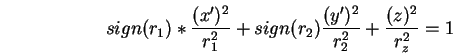
Surfaces that curve in two directions are not well represented here. The problem is that on these surfaces, curvature varies everywhere (except for on a perfect sphere), whereas we would like to characterize the surface simply and globally. Given the segmentation criteria, one feature that does remain constant is the sign of the principal curvatures. To make the characterization more useful, we also include the magnitudes and three dimensional directions of the curvatures at a nominal central point. While this is just an approximation, it is useful for model matching.

When it is necessary to draw or predict instances of these SURFACEs, the model used is ( $r_1 = radius_1, r_2 = radius_2$):

$$sign(r_1) * \frac{(x')^2}{r^2_1} + sign(r_2) \frac{(y')^2}{r^2_2} + \frac{(z)^2}{r^2_z} = 1$$

where $r_z$ = 50 (an arbitrary choice) and $(x',y')$ are in a coordinate system that places $x'$ along the major curvature axis.

Surfaces with twist are neither modeled nor analyzed.

All SURFACEs are presumed to bound solids; laminar surfaces are formed by joining two model SURFACEs back to back. Hence, the normal direction also specifies the outside surface direction.

The extent of a SURFACE is defined by a three dimensional polycurve boundary. The surface patch lies inside the boundary, when it is projected onto the infinite surface. These patches are intended to be only approximate as: (1) it is hard to characterize when one surface stops and another starts on curved surfaces, and (2) surface extraction and description processes do not reliably extract patch boundaries except near strong orientation discontinuities. This implies that surface patches may not smoothly join. However, this is not a problem as the models are defined for recognition (which does not require exact boundaries), rather than image generation.

The polycurve boundary is specified by a few three dimensional points and connecting segments: "point - curve - point - curve - ...". The connecting curve descriptions are either straight lines or portions of circular arcs.

The surface feature that causes the curve or surface segmentation is recorded as part of the model. The surface segmentation boundary labels are (refer to Chapter 3 for their definition):

BN	non-segmenting extremal boundary
BO	surface-orientation
BC	surface-curvature-magnitude
BD	surface-curvature-direction

The curve segmentation point labels are:

PO	boundary-orientation
PC	boundary-curvature-magnitude
PD	boundary-curvature-direction

These labels were not used by the recognition process, but can provide stronger constraints on the identity of surface groupings.

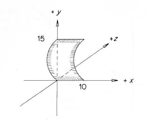
An example of a full SURFACE description of the small curved end surface of the robot upper arm (called "uends") is:

        SURFACE uends = 
            PO/(0,0,0) BC/LINE
            PO/(10,0,0) BO/CURVE[0,0,-7.65]
            PO/(10,15,0) BC/LINE
            PO/(0,15,0) BO/CURVE[0,0,-7.65]
            CYLINDER[(0,7.5,1.51),(10,7.5,1.51),7.65,7.65]
            NORMAL AT (5,7.5,-6.14) = (0,0,-1);

This describes a convex cylinder with a patch cut out of it. The next to last line defines the cylinder axis endpoints and the radii at those points. Here, we see that the axis is parallel to the x-axis. The four lines above that define the polycurve boundary, using four points linked by two line and two circular arc sections. All boundary sections are connected at orientation discontinuities (PO), while the surface meets its neighbors across orientation (BO) and curvature magnitude (BC) discontinuities at the given boundary section. The final line records the direction of the surface normal at a nominal central point. Figure 7.1 shows the surface and boundary specifications combined to model the end patch.

Figure 7.1: Upperarm Small Curved End Patch

ASSEMBLY Definition

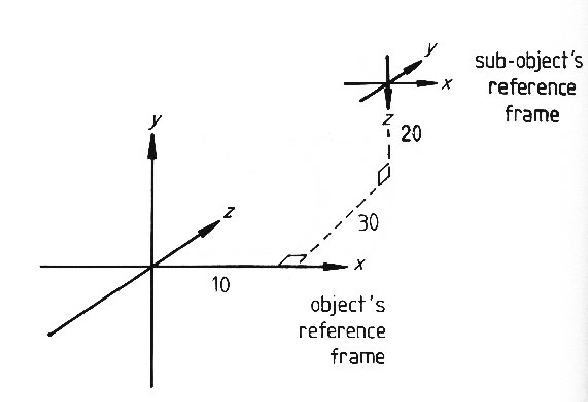
Whole objects (called ASSEMBLYs) are described using a subcomponent hierarchy, with objects being composed of either SURFACEs or recursively defined subcomponents. Each ASSEMBLY has a nominal coordinate reference frame relative to which all subcomponents are located. The geometric relationship of a subcomponent to the object is specified by an AT coordinate system transformation from the subcomponent's reference frame to the object's. This is equivalent to the ACRONYM [42] affixment link. The transformation is specified using an $xyz$ translation and a rotation-slant-tilt reorientation of the subcomponent's coordinate system relative to the ASSEMBLY's. The transformation is executed in the order: (1) slant the subcomponent's coordinate system in the tilt direction (relative to the object's $xy$ plane), (2) rotate the subcomponent about the object's $z$-axis and (3) translate the subcomponent to the location given in the object's coordinates. The affixment notation used in the model definition (Appendix A) is of the form:

$$((trans_x,trans_y,trans_z),(rotation,slant,tilt))$$

Figure 7.2 shows an example of the transformation:

$$((10,20,30),(0,\pi/2,\pi/2))$$

Figure 7.2: Coordinate Reference Frame Transformation

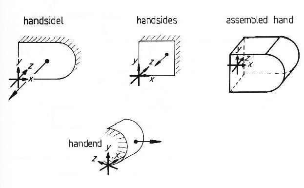
Figure 7.3 shows the robot hand ASSEMBLY defined from three SURFACEs: handsidel (the long lozenge shaped flat side), handsides (the short rectangular flat side) and handend (the cylindrical cap at the end). Assuming that all three SURFACEs are initially defined as facing the viewer, the ASSEMBLY specification is:

        ASSEMBLY hand = 
            handsidel AT ((0,-4.3,-4.3),(0,0,0))
            handsidel AT ((0,4.3,4.3),(0,pi,pi/2))
            handsides AT ((0,-4.3,4.3),(0,pi/2,3*pi/2))
            handsides AT ((0,4.3,-4.3),(0,pi/2,pi/2))
            handend AT ((7.7,-4.3,-4.3),(0,pi/2,0));

Figure 7.3: Robot Hand ASSEMBLY

The SURFACEs do not completely enclose the ASSEMBLY because the sixth side is never seen. This causes no problem; a complete definition is also acceptable as the hypothesis construction process (Chapter 9) would deduce that the SURFACE is not visible when attempting to fully instantiate a hypothesis.

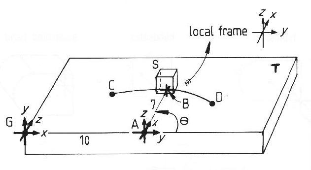
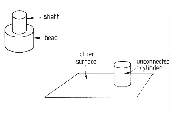
Affixments with degrees-of-freedom are specified by using a FLEX (or SYM) option, which allows unspecified translations and rotations of the subcomponent, in its local reference frame, about the affixment point. The partially constrained attachment definitions use one or more symbolic parameters. The distinction between the FLEX and SYM option is as follows:

• FLEX is used for orientable objects with a partially constrained affixment between them. The variables in the definition are bound to values when the components are linked during recognition.
• SYM is used for unorientable, rotationally symmetric objects. Any value can be matched to the variable during recognition, and the variables always have values during enquiry (nominally 0.0). Examples of this from the models used in this research include the chair legs.

The AT and FLEX (or SYM) transformations are largely equivalent, and so could be algebraically combined, but this complicates the definition task. A subcomponent's partially constrained position is usually specified relative to the subcomponent, not the ASSEMBLY. The affixment to the ASSEMBLY, however, is usually about a point that is defined in the ASSEMBLY's reference frame, so that the two transformations are separated.

An ASSEMBLY S with a rotational degree-of-freedom is shown in Figure 7.4. It is attached to the table T and rotates rigidly (to angle $\Theta$) along the path CD. S and T are part of ASSEMBLY Q. Both T and Q have their coordinate frames located at G and S has its at B. The ASSEMBLY is defined:

        ASSEMBLY Q = 
            T AT ((0,0,0),(0,0,0))     % T is at G
            S AT ((10,0,0),(3*pi/2,pi/2,0)) % from G to A
            FLEX ((-7,0,0),(Theta,0,0));   % from A to B

Figure 7.4: Partially Constrained ASSEMBLY Example

The recursive subcomponent hierarchy with local reference frames supports a simple method for coordinate calculations. Assume that the hierarchy of components is:

        ASSEMBLY P0 =         
            P1 AT A1
            FLEX F1
        ASSEMBLY P1 =
            P2 AT A2
            FLEX F2
        ASSEMBLY P2 =
            P3 AT A3
            FLEX F3
        ...

Let 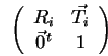$A_i$ and $F_i$ be simplified homogeneous coordinate matrices representing the reference frame transformations given above. Then, each of these 4*4 matrices has the form:

$$\left( \begin{array}{cc} R_i&\vec{T_i}\\ \vec{0}^t&1\\ \end{array}\right)$$

where $R_i$ is the $3 \times 3$ rotation matrix and $\vec{T_i}$ is the translation vector. Each matrix represents the transformation $\vec{T_i} + R_i*\vec{v}$ of a vector $\vec{v}$ in the subcomponent to the object coordinate system. If:

$G$ is the matrix transforming the ASSEMBLY's top level coordinate system
	into global coordinates, and
$C$ transforms from global coordinates into those of the camera,

then a point $\vec{p}$ in the local coordinate system of ASSEMBLY $P_n$ can be expressed in camera coordinates by the calculation:

$$CG(A_1F_1^{-1})(A_2F_2^{-1}) ... (A_nF_n^{-1})\vec{p}$$

There are many ways to decompose a body into substructures, and this leads to the question of what constitutes a good segmentation. In theory, no hierarchy is needed for rigidly connected objects, because all surfaces could be directly expressed in the top level object's coordinate system. This is neither efficient (e.g. there may be repeated structure) nor captures our notions of substructure. Further, a chain of multiple subcomponents with partially constrained affixments represented in a single reference frame would have a complicated linkage definition.

Some guidelines for the decomposition process are:

1. Object surfaces are segmented according to the shape discontinuity criteria of Chapter 3.
2. Non-rigidly connected substructures are distinct ASSEMBLYs.
3. Repeated structures become distinct ASSEMBLYs (e.g. a common surface shape, like a chair leg).
4. Surface groups surrounded by concave surface shape discontinuities become ASSEMBLYs (e.g. where the nose joins to the face). This is because one cannot distinguish a connecting-to from a sitting-on relationship, and so data segmentation must take the conservative choice. Hence, the models should follow this as well. Figure 7.5 illustrates this problem for a structure that might be a rivet or a cylinder on a plane.

Figure 7.5: Segmenting a Rivet Versus a Cylinder on a Plane

Examples of the Models

A range of solid and laminar structures were modeled. The robot model (Figure 1.9) has four rigid subcomponents: the cylindrical base, the shoulder, the upper arm and the lower arm/gripper. Each of these is an ASSEMBLY, as are several of their subcomponents. These four components are joined hierarchically using the FLEX option to represent the partially constrained joint angles. The shoulder body and robot body are defined using non-segmenting boundaries to correspond to the observed extremal boundaries (as discussed below).

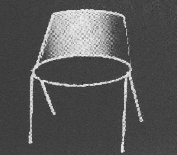
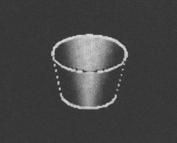
The chair (Figure 7.6) and trash can (Figure 7.7) illustrate laminar surfaces and symmetric subcomponents (SYM). The chair legs are defined as thin cylinders, which are attached by a SYM relation to the chair, as is the seat. The seat and back are both laminar surfaces defined using two back-to-back SURFACEs (with their associated surface normals outward-facing). A similar construction holds for the trash can. Its model has six SURFACEs, because both the outer and inner cylindrical surfaces were split into two, with non-segmenting boundaries joining.

The complete model for the robot is given in Appendix A.

Figure 7.6: Chair Model

Figure 7.7: Trash Can Model

Discussion on the Geometric Model

There are several major inadequacies with the geometric modeling system. Object dimensions have to be fixed, but this was largely because no constraint maintenance mechanism was available (unlike in ACRONYM [42]). Uniform surface and boundary segment curvatures were also simplifications. However, because major curvature changes cause segmentations, deviations between the models and observed objects should be minor. The point was to segment the models in a similar manner to the data, to promote direct feature matching through having a similar representation for both.

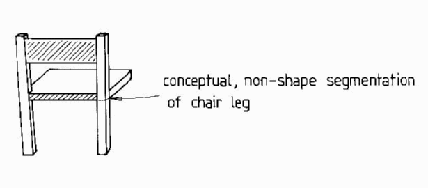
Of course, some surfaces do not segment into conceptual units strictly on shape discontinuities, such as when a chair leg continues upward to form part of the chair back (Figure 7.8). Here, the segmentation requires a boundary that is not in the data. This is part of the more general segmentation problem, which is ignored here.

Figure 7.8: Chair Leg Becomes Part of Chair Back

The surface matching process described in Chapter 9 recognizes image surfaces by pairing them with model SURFACEs. Because non-planar surfaces can curve away from the viewer's line-of-sight, the observed surface patch may not correspond to the full modeled patch. Moreover, extremal boundaries will be seen, and these will not correspond with the patch boundaries.

As the matching process can not properly account for this phenomenon, it was necessary to ensure that the models were defined to help avoid the problem. This required splitting large curved surfaces into patches corresponding to typically obscured surfaces. For example, full cylindrical surfaces were split into two halves, because only one half could be seen from any viewpoint. The new cylindrical patch boundaries approximately correspond to the extremal boundaries (i.e. subset of the front-side-obscuring boundaries) of the observed surface.

For surfaces with an extent that distinguishes orientation, this approach needs extension. A key instance where this splitting was adequate but not general was with the cylindrical robot shoulder, because the shoulder had an irregular notch where it connected to the base. As with the cylindrical surface, the patch was split at its apex to give a boundary that could be matched with the observed extremal boundary, and a roughly corresponding surface patch. If the robot had been viewed from an orientation substantially above or below that actually seen in Figure 1.1, the shoulder patch may not have been recognized.

Surfaces have been represented with a single boundary, and so must not have any holes. The important issues of scale, natural variation, surface texture and object elasticity/flexibility are also ignored, but this is true of almost all modeling systems.

This surface-based representation method seems best for objects that are primarily man-made solids. Many other objects, especially natural ones, would not be well represented. The individual variation in a tree would not be characterizable, except through a surface smoothing process that represented the entire bough as a distinct solid with a smooth surface, over the class of all trees of the same type. This is an appropriate generalization at a higher level of conceptual scale. Perhaps a combination of this smoothing with Pentland's fractal-based representation of natural texture [130] could solve this problem.

According to the goals of the recognition system, an object probably should not be completely modeled, instead only the key features need description. In particular, only the visually prominent surfaces and features need representation and these should be enough for initial identification and orientation.

Finally, any realistic object recognition system must use a variety of representations, and so the surface representation here should be augmented. Several researchers (e.g. [121,42,112]) have shown that axes of elongated regions or volumes are useful features, and volumetric models are useful for recognition. Reflectance, gloss and texture are good surface properties. Viewer-centered and sketch models provide alternative representations.