Property Evidence

Property evidence is calculated by evaluating the fit of structural properties (Chapter 6) to model requirements (Chapter 7). An example of a set of requirements would be a particular surface must be planar and must meet all adjacent connected surfaces at right angles.

There is some controversy over what constitutes evidence, but here, evidence is based only on primitive image properties, such as relative curve orientation, rather than higher level descriptions, such as "rectangular". This decision is partly made because "rectangular" is a distinct conceptual category and, as such, would be included as a distinct generic element in the invocation network. It would then have a description relationship to the desired model.

The context within which data is taken depends on the structure for which property evidence is being calculated. If it is a model SURFACE, then properties come from the corresponding surface hypothesis. If it is an ASSEMBLY, then the properties come from the corresponding surface cluster.

Unary evidence requirements are defined in the model database in one of six forms, depending on whether the values are required or excluded, and whether there are upper, lower or both limits on their range. The complete forms are (where e=evidence_type is the type of evidence):

central include:

UNARYEVID $low$ $<$ e $<$ $high$ PEAK $peak$ WEIGHT $wgt$

above include:

UNARYEVID $low$ $<$ e PEAK $peak$ WEIGHT $wgt$

below include:

UNARYEVID e $<$ $high$ PEAK $peak$ WEIGHT $wgt$

central exclude:

UNARYEVID $low$ $<$ e $<$ $high$ PEAK $peak$ ABSENT WEIGHT $wgt$

above exclude:

UNARYEVID $low$ $<$ e PEAK $peak$ ABSENT WEIGHT $wgt$

below exclude:

UNARYEVID e $<$ $high$ PEAK $peak$ ABSENT WEIGHT $wgt$

If the peak value is the mean of the upper and lower limit, it need not be specified. Each requirement has a weight that scales the contribution of this evidence in the total property evidence evaluation.

Binary evidence requirements are defined similarly, with the key difference that the model also specifies the types of the substructures between which the properties are to hold. The model specification for the binary "central include" form is:

  BINARYEVID low < evidence_type(type1,type2) < high PEAK peak WEIGHT wgt

In IMAGINE I, all evidence types were considered to be unary. If a binary property between two features was expressed, then evidence evaluation would take the best instance of the binary relationship. IMAGINE II made the relationship explicit. The properties used in IMAGINE I were:

NUMLINB	number of straight lines in boundary
NUMARCB	number of curves in boundary
DBPARO	number of groups of parallel lines in boundary
NUM90B	number of perpendicular boundary junctions
NUMEQLB	number of groups of equal length boundary segments
DCURV	boundary segment curvature
DCRVL	boundary segment length
DBRORT	boundary segment relative orientation
MINSCURV	minimum surface curvature
MAXSCURV	maximum surface curvature
SURSDA	relative surface orientation
ABSSIZE	surface area
RELSIZE	percent of surface area in surface cluster
SURECC	eccentricity of surface

It is possible to generate automatically most of the evidence types from the geometric models, if heuristics for setting the ranges and weight values are given, but all these values were manually chosen here. Appendix A shows some of the evidence constraints for the modeled objects.

Models inherit evidence from their descriptions (discussed here), so only additional evidence (i.e. refinements) need be specified here.

Finally, we consider how the total evidence value is calculated from the individual pieces of evidence. The constraints on this computation are:

• Each piece of evidence should contribute to the total value.
• The contribution of a piece of evidence should be a function of its importance in uniquely determining the object.
• The contribution of a piece of evidence should be a function of the degree to which it meets its constraints.
• Negative evidence should inhibit more strongly than positive evidence support.
• Each piece of evidence should only be evaluated by the best fitting constraint (allowing disjunctive evidence constraints).
• All constraints need evidence.
• Every property must meet a constraint, if any constraints of the appropriate type exist.
• Not all properties are constrained (i.e. some are irrelevant).
• Binary property evaluations are also a function of the plausibility that the two substructures have the desired identities.

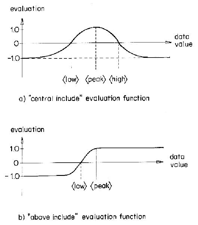
Based on the "degree of fit" requirement, a function was designed to evaluate the evidence from a single description. The function is based on a scaled gaussian evaluation model, with the evaluation peaking at the desired value, having positive value within the required range (which need not be symmetric), and tailing off to -1.0. Because there are six types of evidence requirements, six different evidence evaluation functions are needed. However, the excluded types are the negatives of the included types, and the below types are the mirror image of the above types. So, only the "central include" and "above include" are described here. Based on the model definitions above, the "central include" function for the $i^{th}$ evidence constraint is:

Let;
	$d_j$ = $j^{th}$ data value
If: $d_j > peak_i$
	then: $f_{ij} = (\frac{(d_j - peak_i)}{(high_i - peak_i)} * 1.1774)^2$
	else: $f_{ij} = (\frac{(peak_i - d_j)}{(peak_i - low_i)} * 1.1774)^2$
And the evaluation $e_j$ is:
	$g_{ij} = 2 * exp(-\frac{f_{ij}}{2}) - 1$

The constant 1.1774 ensures the evaluation equals 0 when the data value equals $high$ or $low$. The "above include" function for the $i^{th}$ evidence constraint is:

Let:
	$d_j$ = $j^{th}$ data value
If: $d_j > peak_i$
	then: $f_{ij} = 0.0$
	else: $f_{ij} = (\frac{(peak_i - d_j)}{(peak_i - low_i)} * 1.1774)^2$
And the evaluation $e_j$ is:
	$g_{ij} = 2 * exp(-\frac{f_{ij}}{2}) - 1$

Figure 8.7 illustrates these functions. Their gaussian form is appealing because it is continuous and smooth and relates well to gaussian error distributions from property estimation. Other functions meet the requirements, but stronger requirements could not be found that define the function more precisely.

Figure 8.7: Data Evaluation Functions

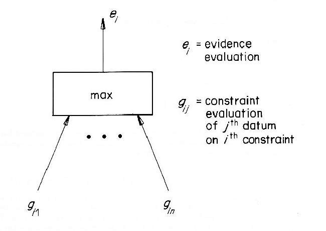
A property constraint's evaluation is given by the data value that best satisfies the constraint. This is because model-to-data correspondences have not been made yet, so the evaluations are undirected. As the point of invocation is suggestion, any datum within the constraint range is contributory evidence, and correct models will have all their constraints satisfied. Hence, the final evidence value for this constraint is given by:

$$e_i = max_j(g_{ij})$$

This portion of the invocation network is illustrated in Figure 8.8.

Figure 8.8: Best Evaluation Selection Network Fragment

The evaluation of binary property evidence takes into account the plausibility of the subcomponents as well as the property value itself. Thus:

$$h_{abi} = c_1 * g_i(a,b) + c_2 * p_{ar} + c_2 * p_{bs} + c_3$$

is the evidence evaluation function for the $i^{th}$ binary evidence constraint, relating model subcomponent $r$ to model subcomponent $s$, when using the value of the given property between data features $a$ and $b$. $g_i(a,b)$ is the same evaluation function as for the unary properties ($g_{ij}$), $p_{ar}$ and $p_{bs}$ are the plausibilities that data feature $a$ has model identity $r$, data feature $b$ has model identity $s$, and $c_1$, $c_2$ and $c_3$ are constants that express the relative importance of the different terms ( $c_1 = 0.8, c_2 = 0.4, c_3 = -0.6$). The final binary property evidence value is:

$$e_i = max_{ab}(h_{abi})$$

This picks the best evidence over all pairs of immediate subfeatures in the data context.

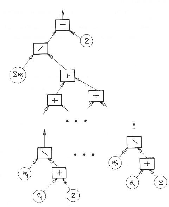
The evaluations for individual property requirements then need to be integrated. One function that satisfies the evidence integration constraints is a weighted harmonic mean:

let:
	$e_i$ be the data evaluation for the $i^{th}$ property constraint
	$w_i$ be the weight for that evidence type
Then:
	$evd_{prop} = harmmean(\{(e_i,w_i)\})$
where
	$A = \sum w_i$
	$B = \sum \frac{w_i}{e_i + 2}$
	$harmmean(\{(e_i,w_i)\}) = \frac{A}{B} - 2$

If no property evidence is available, this computation is not applied. The modified harmonic mean is continuous, gives additional weight to negative evidence and integrates all values uniformly. Moreover, it has the property that:

$harmmean(\{(e_1,w_1),(e_2,w_2),(e_3,w_3)\})$

$= harmmean(\{(e_1,w_1), (harmmean(\{(e_2,w_2),(e_3,w_3)\}),w_2+w_3)\})$

This means that we can add evidence incrementally without biasing the results to the earlier or later values (provided that we also keep track of the weighting of the values). The offset of 2 is used to avoid problems when the plausibility is near -1, and was chosen because it gave good results. The integrated property evidence has a weight that is the sum of the individual property weights: $w_{prop} = \sum w_i$.

This harmonic mean can be implemented in a value passing network, as shown in Figure 8.9, which integrates the evidence values $e_i$ with weights $w_i$. Here, the square boxes represent unary or binary arithmetic units of the designated type, and circular units represent either constants, or the evidence values imported from the above calculation.

Figure 8.9: Harmonic Mean Network Fragment Integrating Property Evidence