Experimental Results

In this section, we briefly describe the experiments conducted to calibrate two Hitachi HP-M1 CCD cameras with H10x11E Fujinon active lenses that are part of a trinocular active-vision system developed at our lab. The lens of these cameras has focal length 11mm - 110mm, focus range $\infty$ - 1.2m and iris range F1.9 - F22. The lens has 3 motors for iris, zoom and focus control. However, except for the iris motor, each of the other two motors provides a position reading presented as a dc voltage in the range 0 - 16384 after A/D conversion. In the following, we will refer to this range in normalized presentation from 0 - 1. For the operating range,we have chosen a focus range of $0.5 \le m_f < 1.0$ which corresponds roughly to a focused distance of 1.2m to 2.5m. For the zoom, we have chosen a similar range of $0.5 \le m_z < 1.0$ which corresponds to focal length from approximately 11mm up to 25mm, while the iris is kept wide-open. We used a regular 7 x 7 sampling of the selected zoom and focus ranges. At each lens setting, an image was captured by the camera of a chessboard-like calibration pattern, thus a total of 49 sets of calibration data were obtained. Each set contained 440 data points. The calibration approach, explained in Section 4, was applied to the collected calibration data of each camera independently. In the global optimization stage, the networks were trained until the root mean square (rms) of calibration error dropped below 0.1 pixels, and the rms of fitting error for each parameter MLFN was below 0.1. Figure 2 illustrates some of the obtained parameter variations versus zoom and focus settings.

Figure 2:Variations of some model parameters versus normalized focus and zoom settings of one lens:(a)$u_0$(pix.), (b) t_y(cm), (c) t_z(cm) and (d) $\alpha _u$(pix.).

For comparison sake, we applied Wilson's approach [14] to the same collected calibration data (but using the camera model in Section 2 instead of Tsai's [11]). Table II summarizes the order of bivariate polynomials selected for our implementation of Wilson's approach and the MLFN topologies chosen to model the zoom and focus varying parameters. Note that a bivariate polynomial of order $q$ has $(q+1)(q+2)/2$ coefficients.

Table II:Polynomial orders and network topologies used to fit the zoom and focus varying parameters.

Parameter	poly. order	Net topology
tz	5	2-5-1
$u_0$	3	2-3-1
$v_0$	3	2-3-1
$\alpha _u$	6	2-5-2-1
$\alpha_v$	6	2-5-2-1

In the global optimization step using the Levenberg-Marquardt algorithm in Wilson's approach [14], the order of fitting the parameter polynomials to the data affects the final calibration error. Therefore, as Wilson suggested, the polynomial coefficients of lowest order were optimized first followed by the higher ones in increasing order, using a greedy algorithm whenever two or more parameter models have the same polynomial order. The rms of calibration error in pixels is shown in Table III for the two cameras, computed over all 49 x 440 data points, before and after the global optimization step for the two methods.

Table III:Comparison of the rms of calibration error in pixels before and after global optimization between our proposed approach and Wilson's.

	Camera 1		Camera 2
Approach	Init	Fin	Init	Fin
Wilson's	5.4	1.8	6.2	1.3
Ours	2.5	0.1	1.8	0.1

Since we have not imposed on the calibration procedure the fact that the aspect ratio, $\alpha_v/\alpha_u$, should be nearly constant (from our earlier experience with these cameras, it is equal to 1) across the different lens settings, we used this to assess the results of our calibration. Our results, for both cameras, have shown a aspect ratio of $1\pm 0.05$ across all zoom and focus calibrated ranges. Moreover, since the two cameras that we used form a stereo rig and we often captured images of the same calibration patterns by both of them, one can compute for these images the rms of the error in 3D reconstruction of the calibration pattern. This will serve as a quantitative measure of calibration accuracy. Table IV shows this measure computed, using 20 images, for the two approaches using the calibrated parameters before and after the global optimization step. In fact, we have used this measure to validate the different parameter models and to circumvent over/under-fitting given the the size of the available data. Several experiments were necessary before we reached the previous models given in Table II. The calibration accuracy can be further improved if the images are corrected for lens distortion before calibration. Moreover, we can make use of more sampling positions (and thus more collected data size) to improve the accuracy.
 
 

Table IV:Rms of 3D reconstruction error in cm before and after global optimization.

Approach	Initial	Final
Wilson's	2.65	0.91
Ours	1.41	0.32

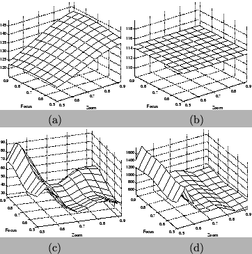
One can read from the above two tables the importance of the global optimization step to improve the calibration error. This step optimizes and refines the parameter-formulated functions taking into account the interaction and correlation between the different model parameters, which combine together to compose the camera projective transformation. This interaction is clearly absent in the function formulation step. The second thing to read from the tables is that our approach has been more able to capture the variations of the parameters across the lens settings. Rather than bivariate polynomials, other alternatives such as Chebyshev polynomials and Legendre polynomials could have been utilized. However, we resort to proven power of MLFNs [3] to provide a suitable parameter formulation. The last point that we like to emphasize is that even if MLFNs are used to provide this function mapping, the role of the neurocalibration network remains important to form an effective framework to optimize and refine these function mappings towards more accurate calibration results.