


One approach to locating examples of objects whose shape can vary
(eg faces or internal organs) is to use Active Shape Models [21].
This method relies on building a statistical model of shape variation from
examples in a training set. Each example object is represented using a
fixed number of landmark points 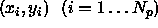 , each of which
marks a particular point on the object. The training examples are aligned
into a common co-ordinate frame and each is then represented by a
, each of which
marks a particular point on the object. The training examples are aligned
into a common co-ordinate frame and each is then represented by a  element vector
 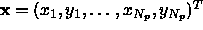 .
If we make the assumption that such vectors have a gaussian distribution
for the training set we can build a linear model as follows
.
If we make the assumption that such vectors have a gaussian distribution
for the training set we can build a linear model as follows

where  is the mean of the training set, b is
a vector of t shape parameters and P is a
is the mean of the training set, b is
a vector of t shape parameters and P is a  x t matrix
formed from the t principle eigenvectors of the covariance matrix of
the training set. The t shape parameters,
x t matrix
formed from the t principle eigenvectors of the covariance matrix of
the training set. The t shape parameters,  , are then mutually
independent and the
, are then mutually
independent and the  is gaussian with zero mean and variance
 (the
(the  largest eigenvalue of the covariance matrix).
See [21] for details.
largest eigenvalue of the covariance matrix).
See [21] for details.
For instance Figures 6 and 7 show the effects of varying two of the parameters of a face model which uses 169 points to represent the shape of various facial features.
Figure 6: Effect of varying shape parameter 1 of 169 point face model
Figure 7: Effect of varying shape parameter 2 of 169 point face model
To find the best fit of an instance of such a model to a new image,
we must find the shape parameters, b, position,  ,
orientation,
,
orientation,  , and scale, s, which best match the model to
the image. Once again, defining a suitable objective function is
difficult. The method used in the Active Shape Model is as follows.
, and scale, s, which best match the model to
the image. Once again, defining a suitable objective function is
difficult. The method used in the Active Shape Model is as follows.
We first must determine how well each individual model point matches
the image, when placed at a particular location. For each model point
we build a statistical model of the intensity variation in a region
about each point, using the training set (section 3.2.1).
This allows us to find a point in the image  which best
matches the
which best
matches the  model point, by searching a region around the
current position
model point, by searching a region around the
current position  .
A good model position would have each point near to its corresponding
best match, leading to an objective function of the form
.
A good model position would have each point near to its corresponding
best match, leading to an objective function of the form

where  is the distribution of location error. Because the model (
 ) is a truncated approximation, it will not fit
exactly to all plausible object shapes.
) is a truncated approximation, it will not fit
exactly to all plausible object shapes.
If we assume a gaussian distribution of point position errors, then a
straightforward least squares method can be used to find the optimal
parameters  for a given set of best match
points
for a given set of best match
points  .
.
Remember, however, that the best match points are obtained by searching around the current position for each model point. If the model points are not near the correct position then some of the matches will not be optimal, simply because the region searched did not include the true position for the point. The hope is that enough points were matched well, so that the new set of parameters moves the model points closer to the true solution. We thus use an iterative approach to solving the problem:
REPEAT
 calculate positions
of model points,
calculate positions
of model points,  .
.
 for the best match of
a corresponding region model,
for the best match of
a corresponding region model, 

When the starting point is `close enough' to the true image object, this algorithm will usually converge successfully. Its performance can be improved by using a multi-resolution framework in which the earlier iterations are performed using low resolution versions of the local region models searching on a low resolution version of the image [22]. For instance, Figure 8 shows the face model iterating to fit a face image.
Notice that we could attempt to locate the optima by applying a local
minimizer (eg Simplex) to  . This would
be very expensive since most of the work involved is in locating the best
nearby matches for each model point, which would have to be done for every
new function evaluation. The algorithm above attempts to make better use
of the match information, updating the parameters effectively after every
function evaluation. This approach of breaking a model matching
problem into a series of independent local searches, followed by a
parameter update (or regularization) stage is often used for Active
Contour Models (`Snakes') and is discussed in detail by Cohen [23].
. This would
be very expensive since most of the work involved is in locating the best
nearby matches for each model point, which would have to be done for every
new function evaluation. The algorithm above attempts to make better use
of the match information, updating the parameters effectively after every
function evaluation. This approach of breaking a model matching
problem into a series of independent local searches, followed by a
parameter update (or regularization) stage is often used for Active
Contour Models (`Snakes') and is discussed in detail by Cohen [23].
Notice that in the definition of the objective function only the position
of the local model matches is used, not their quality. In theory, since
we have a statistical model of the expected intensity variation for each
match, we can assign a likelihood,  , that the match is correct.
We could then generate an objective function of the form
, that the match is correct.
We could then generate an objective function of the form
However, this cannot be minimized using the two stage algorithm given above, and we must resort to the more expensive general methods.
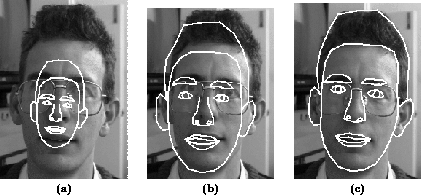
Figure 8: a) Initial Position b) After 10 iterations c) At convergence of ASM search