Evaluation

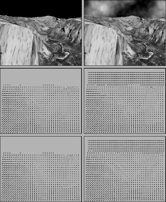
For evaluation of the method we use the famous Yosemite sequence with and without cloudy sky. The original version with cloudy sky was created by Lynn Quam and is available at ftp://ftp.csd.uwo.ca/pub/vision. It combines both divergent and translational motion. The version without clouds is available at http://www.cs.brown.edu/people/black/images.html.
The flow fields obtained with the method are presented in Fig.1 They match the ground truth very well. Not only the discontinuity between the two types of motion is preserved, also the translational motion of the clouds is estimated accurately. The reason for this behaviour lies in the model assumptions, that are clearly stated in the energy functional: While the choice of the smoothness term allows discontinuities, the gradient constancy assumption is able to handle brightness changes - like in the area of the clouds.

Figure 1: (a) Top left: Frame 8 of the Yosemite sequence without clouds. (b) Top right: Corresponding frame of the sequence with clouds. (c) Middle left: Ground truth without clouds. (d) Middle right: Ground truth with clouds. (e) Bottom left: Computed flow field by our 3D method for the sequence without clouds. (f) Bottom right: Ditto for the sequence with clouds.

Noise
Because of the presence of second order image derivatives in the Euler-Lagrange equations, the influence of noise on the performance of the method is tested in another experiment. We added Gaussian noise of mean zero and different standard deviations to both sequences. The obtained results are presented in Tab.1. They show that the approach even yields excellent flow estimates when severe noise is present.

Table 1: Results for the Yosemite sequence with and without cloudy sky. Gaussian noise with varying standard deviations $\sigma _n$ was added, and the average angular errors and their standard deviations were computed. AAE = average angular error. STD = standard deviation.

$\sigma _n$

AAE

STD

$\sigma _n$

AAE

STD

0

1.94$^{\circ}$

6.02$^{\circ}$

0

0.98$^{\circ}$

1.17$^{\circ}$

10

2.50$^{\circ}$

5.96$^{\circ}$

10

1.26$^{\circ}$

1.29$^{\circ}$

20

3.12$^{\circ}$

6.24$^{\circ}$

20

1.63$^{\circ}$

1.39$^{\circ}$

30

3.77$^{\circ}$

6.54$^{\circ}$

30

2.03$^{\circ}$

1.53$^{\circ}$

40

4.37$^{\circ}$

7.12$^{\circ}$

40

2.40$^{\circ}$

1.71$^{\circ}$

Parameter robustness
In a third experiment the robustness of the free parameters is tested: the weight $\gamma$ between the grey value and the gradient constancy assumption, and the smoothness parameter $\alpha$. Often an image sequence is preprocessed by Gaussian convolution with standard deviation $\sigma$ [4]. In this case, $\sigma$ can be regarded as a third parameter. Results are computed with parameter settings that deviate by a factor 2 in both directions from the optimum setting. The outcome listed in Tab. 2 shows that the method is also very robust under parameter variations.

Table 2: Parameter variation for our method with spatio-temporal smoothness assumption.

	$\sigma$		$\alpha$		$\gamma$				AAE
	0.8		80		100				$1.94^\circ$
	0.4		80		100				$2.10^\circ$
	1.6		80		100				$2.04^\circ$
	0.8		40		100				$2.67^\circ$
	0.8		160		100				$2.21^\circ$
	0.8		80		50				$2.07^\circ$
	0.8		80		200				$2.03^\circ$

Convergence behaviour
The implicit minimisation scheme presented here is also reasonably fast, especially if the reduction factor $\eta$ is lowered or if the iterations are stopped before full convergence. The convergence behaviour and computation times can be found in Tab. 3. Computations have been performed on a 3.06 GHz Intel Pentium 4 processor executing C/C++ code.

Table 3: Computation times and convergence for Yosemite sequence with clouds.

2D - spatial method

	reduction factor	outer fixed point iter.	inner fixed point iter.	SOR iter.	computation time	AAE
	0.95	77	5	10	16.8s	$2.46^\circ$
	0.85	25	2	10	2.5s	$2.57^\circ$
	0.80	18	1	10	1.1s	$3.55^\circ$
	0.75	14	1	5	0.6s	$4.21^\circ$

3D - spatio-temporal method

	reduction factor	outer fixed point iter.	inner fixed point iter.	SOR iter.	computation time	AAE
	0.95	77	5	10	23.4s	$1.94^\circ$
	0.90	38	2	10	5.1s	$2.09^\circ$
	0.80	18	2	10	2.7s	$2.56^\circ$
	0.75	14	1	10	1.2s	$3.44^\circ$

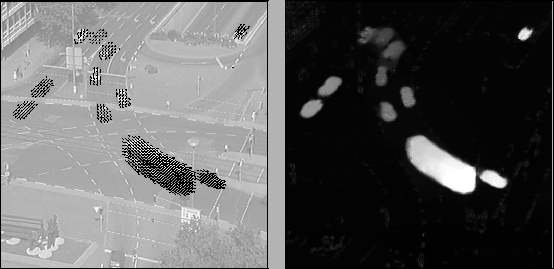
For evaluating the performance of the method with real-world image data, the Ettlinger Tor traffic sequence by Nagel is used. This sequence consists of 50 frames of size $512 \times 512$. It is available at http://i21www.ira.uka.de/image_sequences/. In Fig. 2 the computed flow field and its magnitude are shown. The estimation gives very realistic results, and the algorithm hardly suffers from interlacing artifacts that are present in all frames. Moreover, the flow boundaries are rather sharp and can be used directly for segmentation purposes by applying a simple thresholding step.
The MPEG-files show the original sequence and the computed flow field in a colour code that is overlaid above the images. The hue expresses the direction of motion and the intensity of the colour shows the magnitude of the flow vector.

Figure 2: (a) Left: Computed flow field between frame 5 and 6 of the Ettlinger Tor traffic sequence. (b) Right: Computed magnitude of the optical flow field.

	Original sequence (MPEG,1MB)		Computed flow (MPEG,2.3MB)
	Small version (MPEG,0.5MB)		Small version (MPEG,1.2MB)