Next: Evaluation
Up: Minimisation
Previous: Euler-Lagrange Equations
The preceding Euler-Lagrange equations are nonlinear in their
argument
 . A first step towards a linear system
of equations, which can be solved with common numerical methods, is the
use of fixed point iterations on
. A first step towards a linear system
of equations, which can be solved with common numerical methods, is the
use of fixed point iterations on
 . In order to implement a
multiscale approach, necessary to better approximate the global optimum of
the energy, these fixed point iterations are combined with a downsampling
strategy.
Instead of the standard downsampling factor of
. In order to implement a
multiscale approach, necessary to better approximate the global optimum of
the energy, these fixed point iterations are combined with a downsampling
strategy.
Instead of the standard downsampling factor of  on each level, it
is proposed here to use an arbitrary factor
on each level, it
is proposed here to use an arbitrary factor
 , what allows
smoother transitions from one scale to the next. Moreover, the full
pyramid of images is used, starting with the smallest possible image at
the coarsest grid. Let
, what allows
smoother transitions from one scale to the next. Moreover, the full
pyramid of images is used, starting with the smallest possible image at
the coarsest grid. Let
 ,
,
 ,
with the initialisation
,
with the initialisation
 at the coarsest grid.
Further, let
at the coarsest grid.
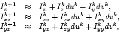
Further, let  be the abbreviations defined in (8)
but with the iteration variable
be the abbreviations defined in (8)
but with the iteration variable
 instead of
. Then
instead of
. Then
 will be the solution of
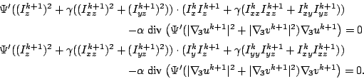 |
(9) |
As soon as a fixed point in
is reached, we change to the next finer
scale and use this solution as initialisation for the fixed point iteration
on this scale.
Notice that we have a fully implicit scheme for the smoothness term and a
semi-implicit scheme for the data term. Implicit schemes are used to yield
higher stability and faster convergence. However, this new system is still
nonlinear because of the nonlinear function  and the symbols
 .
In order to remove the nonlinearity in , first order Taylor
expansions are used:
.
In order to remove the nonlinearity in , first order Taylor
expansions are used:
where
 and
and
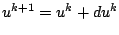
 . So we split the
unknowns
. So we split the
unknowns  ,
,  in the solutions of the previous iteration step
 and unknown increments
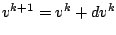
 . For better readability let
 |
(10) |
where
 can be interpreted as a robustness factor in the
data term, and
can be interpreted as a robustness factor in the
data term, and
 as a diffusivity in the smoothness
term. With this the first equation in system (9) can be
written as
as a diffusivity in the smoothness
term. With this the first equation in system (9) can be
written as
and the second equation can be expressed in a similar way.
This is still a nonlinear system of equations for a fixed  , but now
in the unknown increments
. As the only remaining nonlinearity
is due to , and
, but now
in the unknown increments
. As the only remaining nonlinearity
is due to , and  has been chosen to be a convex function,
the remaining optimisation problem is a convex problem, i.e. there exists
a unique minimum solution.
has been chosen to be a convex function,
the remaining optimisation problem is a convex problem, i.e. there exists
a unique minimum solution.
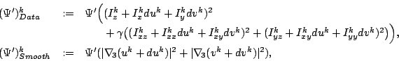
In order to remove the remaining nonlinearity in , a second, inner,
fixed point iteration loop is applied. Let
 ,
,
 be our initialisation and let
 denote the iteration
variables at some step
denote the iteration
variables at some step  . Furthermore, let
 and
and
 denote the robustness
factor and the diffusivity defined in (10) at iteration ,
.
Then finally the linear system of equations in
denote the robustness
factor and the diffusivity defined in (10) at iteration ,
.
Then finally the linear system of equations in
 reads
reads
for the first equation.
Using standard discretisations for the derivatives, the resulting sparse
linear system of equations can now be solved with common numerical methods,
such as Gauss-Seidel or SOR iterations. Expressions of type
 are computed by means of bilinear interpolation.
Next: Evaluation
Up: Minimisation
Previous: Euler-Lagrange Equations
Thomas Brox
2004-06-29