Main Steps of the Method

Our method assumes that the images has been normalized and binarized. Normalization, in this context, is geometric correction of an image. Its purpose is twofold:

• Correct image distortions resulting from the possible deficiencies of the optical setup (camera, lens, viewing geometry).
• Normalize the size of the image for system calibration (pixel/mm ratio).

The normalization is done by mapping onto the image corners the centroids of four circular markers located close to the corners. (See figure 3.) This procedure and the subsequent binarization (thresholding) are presented in [6]. The measurements are done with subpixel accuracy, as described in the same paper. Examples of measurements as well as the dimensions measured in case of E-cores are given in section 4.2.

Note that the our original version of the matching algorithm presented in [6] has a limited scope. Since this algorithm was created for specific products, E-cores, extending this algorithm to other shapes requires complete re-writing of the system. In addition, the original matching algorithm [6] cannot be extended to 3D. The new general matching methodology presented here is free of these deficiencies.

The main steps of the new matching method are as follows.

Step 1

Find contour points of the reference shape and obtain their DT.

Step 2

Obtain contour points of the measured shape.

Step 3

Compute and superimpose the centroids of the two point sets.

Step 4

Rotate and translate the measured point set with respect to the initial pose. For each relative pose, compute the median HD (2) using the corresponding distance values. To speed up, use a distance limit and discard a pose if a measured point is beyond the limit.

Step 5

Select those relative positions that yield the minimum HD value. (Multiple minima are possible.)

Step 6

Of these, select the one that has the least mean HD.

Step 6 resolves ambiguities arising from the integer approximation of the distance. Also, it discards possible false minima when symmetric contours are matched. For such contours, many points may coincide in a wrong orientation because of symmetry, while the rest of the points may not coincide at all.

Alternatively to the criterion of step 6, the pose with the largest number of measured points lying within the minimum median HD can be used.

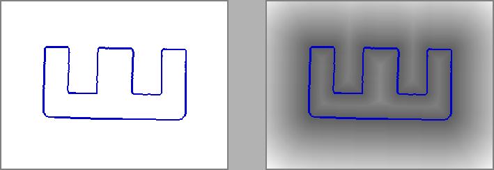
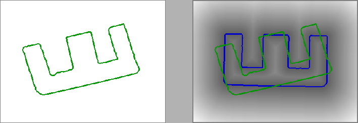
Figures 6 and 7 illustrate the operation of the matching algorithm. Step 1 is exemplified in figure 6, where the contour of a reference ferrite core is shown along with its distance transform. Figure 7 explains the matching of a measured contour against the reference contour of figure 6. In this figure, the measured contour is shown in one of the relative positions, overlaid on the DT of the reference contour. (Step 4.)

  

Figure 6: A reference contour and its DT.

  

Figure 7: A measured contour and the DT of the reference contour with the measured contour overlaid.